Central question: what must a surface do to the electromagnetic field, and how can we tell whether it has done it?
A field crosses from glass into air and its transmitted electric amplitude grows to 1.2 times the incident amplitude. A lossless interface leaves a transmitted field on the other side while transmitting no net normal power. A sheet that absorbs at most half of a single incident beam absorbs all of two suitable beams. None of these statements violates energy conservation. Each asks us to distinguish a field from a power, a local field from a propagating channel, or one illumination from another.
These are our three puzzles. Make an initial prediction for each, then return to them after working through the chapter. The browser lab lets you vary the experiments without installing software; the executed notebook exposes their equations and checks. The worked examples and self-check provide a second path through the same ideas.
2.1 A route through the prerequisites
By the end of this chapter, you should be able to derive rather than memorize the flat-interface response; calculate its power with the correct admittance; distinguish propagation, evanescence, and grazing cutoff; express coherent polarization states with Jones vectors; and decide whether proposed scattering coefficients could describe a stated sheet.
| Stop | Question to predict | Tool to develop |
|---|---|---|
| Waves | Which way does energy travel? | Phasors, , , and Poynting flux |
| Polarization | Can intensity stay fixed while the field changes? | Relative component phase and Jones matrices |
| An interface | Can $ | t |
| Critical angles | Can a field exist without carrying normal power away? | Complex longitudinal wavevector |
| A film | Can adding material reduce reflection? | Coherent interference and phase reference |
| A sheet | Can phase change absorption? | Surface current, scattering channels, and coherence |
Keep a small record beside every calculation: illumination, material model, basis, time convention, reference planes, and power denominator. This is the foundation for every later unit-cell library, diffraction efficiency, and learned response in the book.
2.2 Give a wave a direction
We use real physical fields obtained from complex phasors:
Thus a positive real with travels toward positive . At a fixed phase, is constant. A complex with instead contributes : it decays into the positive- half-space. Choosing the opposite square-root branch would make it grow away from a passive interface.
Maxwell’s equations in a homogeneous source-free region become
Substituting the plane-wave form gives
For a complex wavevector, this dispersion relation uses , rather than . The distinction matters for an evanescent wave.
For a propagating wave in our nonmagnetic real-index media,
The magnetic field is fixed by the electric field and propagation direction. It cannot be assigned an independent sign. In particular, reversing the propagation direction reverses the relevant electric-to-magnetic relation. That sign creates the term in the interface derivation below.
2.3 A field is not a power meter
For phasors defined as peak amplitudes, the time-averaged power-flux density is
The factor belongs to the peak-amplitude convention. For a normally incident propagating wave in a real medium,
An electric amplitude therefore does not have the same power weighting in two different media. A transmitted amplitude of 1.2 in air can carry less power than an incident amplitude of 1 in glass. At oblique incidence, the normal flux and chosen field component introduce additional factors; we will collect them in a wave admittance.
Power is only one observable. The fields and have equal transmitted power in the same normalization, but they interfere differently with a fixed reference. Always retain amplitude and phase together when the design concerns a complex wavefront.
2.4 Make polarization visible
At a fixed point, the tip of the transverse electric field can trace a line, ellipse, or circle over one period. Write a unit-norm Jones vector for propagation along positive as
Here controls the component magnitudes and is the relative phase of with respect to . At ,
For , the vector remains on a line. For and , the normalized state is : starting at positive , the tip moves toward positive as time increases. This description specifies the axes and time convention without relying on a potentially ambiguous handedness label.
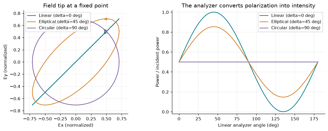
Relative phase changes the field trajectory even when the total Jones-vector norm stays fixed. State the time convention and viewing axes before assigning a handedness name.
An ideal retarder aligned with the axes can have
It changes relative phase while preserving power in this ideal model. An analyzer with real unit axis transmits the fraction
For linear input this becomes Malus’s law; for a normalized circular state it is for every analyzer angle. These are coherent, fully polarized models. A single Jones vector does not represent unpolarized or partially coherent light. Chapter 5 builds ideal Jones transformations; a physical element still needs conversion and leakage data.
2.5 Ask what is continuous
Place the interface at , with unit normal pointing from region 1 to region 2. Integrating the curl equations across an infinitesimal loop gives the tangential jump conditions
is an electric surface-current density in A/m. is an equivalent magnetic surface-current density in V/m under this sign convention; it is a useful field-equivalence description, not a requirement for literal magnetic monopoles. With neither surface current, the tangential electric and magnetic fields are continuous. Normal components satisfy the corresponding flux laws; tangential continuity does not mean every Cartesian component of every field is continuous.
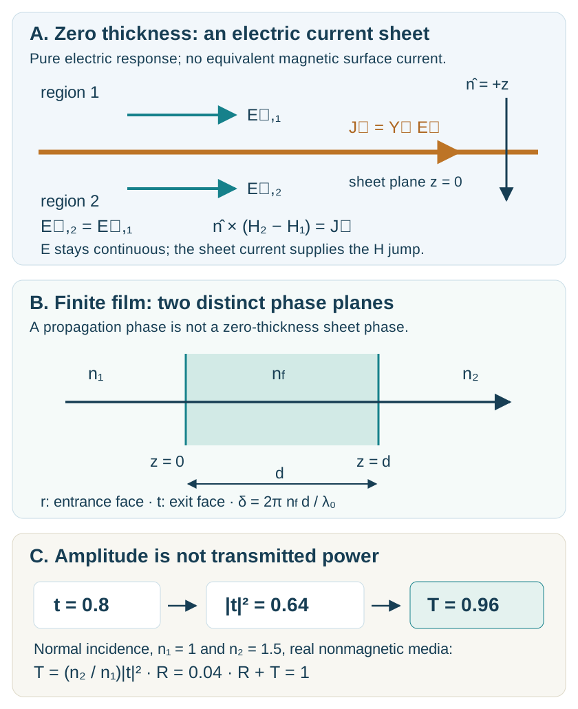
Boundary conditions connect a field transformation to the current needed to support it. The local electric shunt considered here is one restricted example; general tensor, magnetic, and bianisotropic sheet synthesis requires additional relations.
The entire planar interface has the same boundary relation at every . The incident, reflected, and transmitted fields must therefore have matching tangential phase factors:
This is phase matching and, for propagating transmission, Snell’s law. A periodic surface can add reciprocal-lattice wavevectors, as developed in Chapter 4. A desired phase profile is consequently a scattering specification, not a replacement for Maxwell’s boundary conditions.
2.6 Derive the interface response
Take the plane of incidence to be . TE has electric field along . TM has magnetic field along and electric field in the plane. We compare the same tangential electric component on each side: for TE and for TM. Define
choosing the outgoing/decaying root, with nonnegative real and imaginary parts for these lossless positive-index half-spaces. Our dimensionless tangential wave admittance is
The physical admittance is . To see the signs, use the signed tangential magnetic component for TE and for TM. A forward wave has ; a backward wave has the opposite relation. With incident tangential electric amplitude one, continuity gives
Solving these two equations yields the Fresnel coefficients in our basis:
For a propagating incident channel, is real and positive. Its normal power fractions are
For a lossless single interface, . At normal incidence, for both polarizations: from air to glass, , , , and .
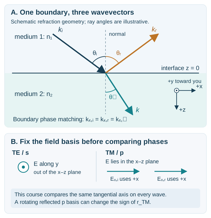
The geometry, polarization basis, and reference plane are part of the definition of a scattering coefficient. Positive normal power leaves the interface into the transmitted half-space.
2.7 Brewster, evanescence, and cutoff
For nonmagnetic dielectric media, TM reflection vanishes when the two TM admittances match. Substituting Snell’s law gives
For air to glass, . The TE wave at that angle still reflects. Brewster cancellation is polarization dependent; it does not say that every field at that interface is reflectionless.
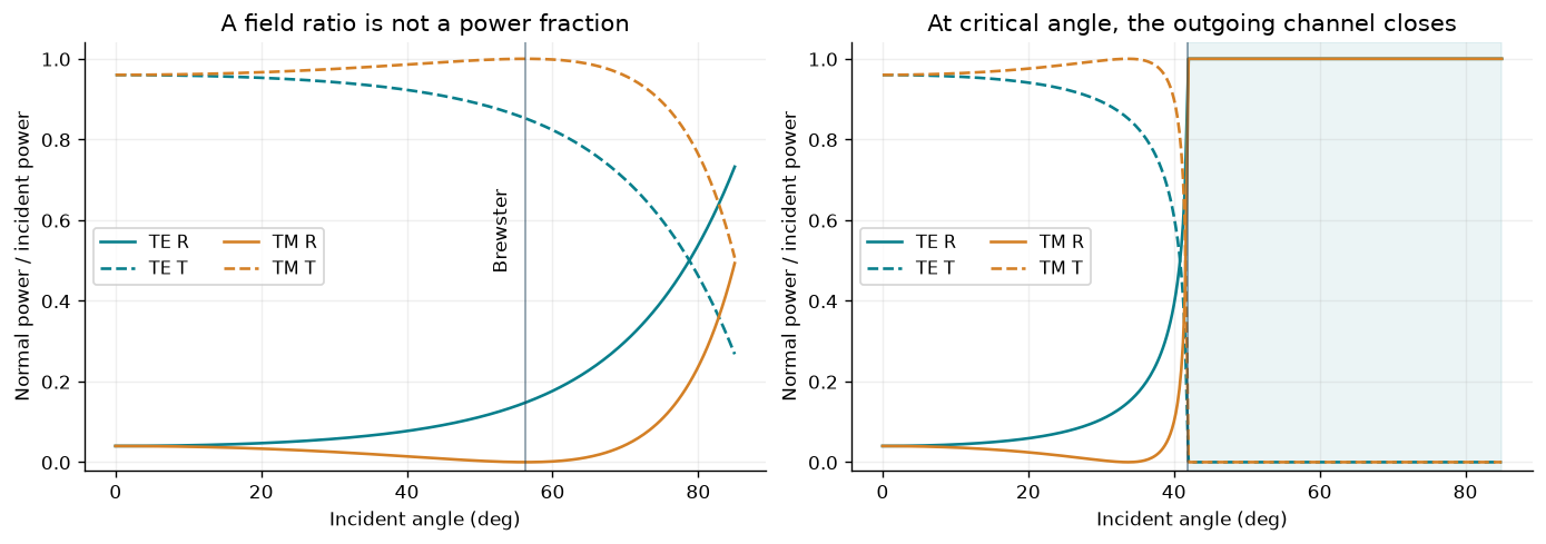
Keep field coefficients and normal power separate. The same admittance expressions account for ordinary refraction, the TM reflection zero, and total internal reflection within their stated domain.
If , the critical angle satisfies . For glass to air, . Above it,
The transmitted field can be nonzero while , giving and . Its amplitude decay length is ; the intensity decay length is half as large. It is incorrect to interpret as proof that the entire transmitted field vanishes. It is also incorrect to interpret a nonzero evanescent amplitude as a nonzero outgoing normal-power channel.
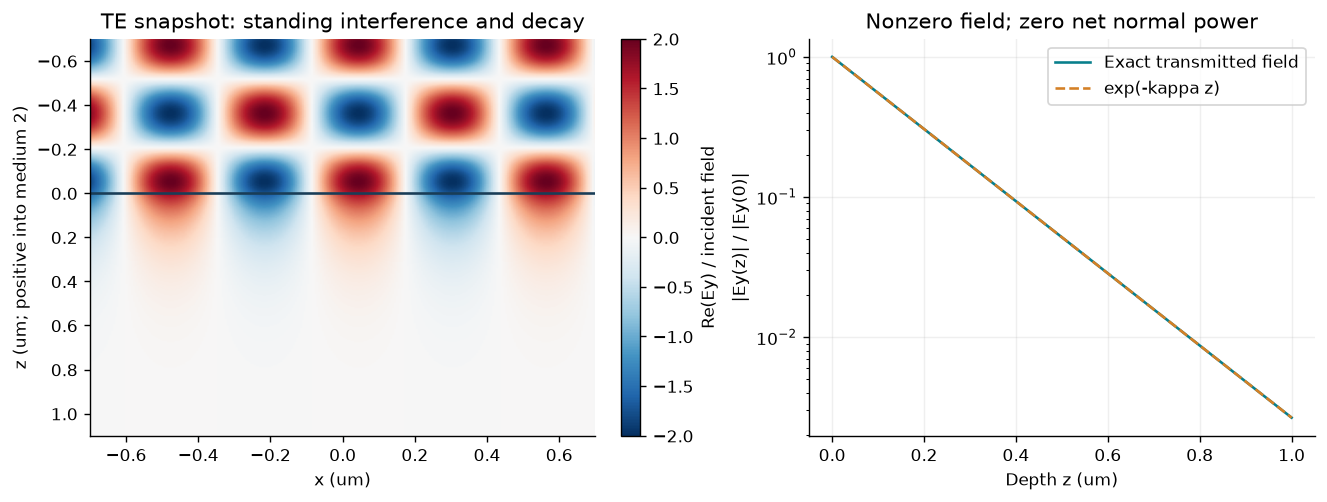
The field penetrates the second medium while its net transmitted normal power is zero for this single, semi-infinite lossless interface. Adding another nearby interface would define a different tunneling problem.
At exact grazing cutoff, formulas containing need limiting treatment. For TM, defined from tangential tends to zero, but the factor relating to can diverge so that the complete transmitted field need not vanish. Approach cutoff from either side and report it separately; do not evaluate a singular intermediate admittance as if it were an ordinary finite propagating channel.
2.8 Add a film and keep the phase
Can adding a material layer reduce reflection? At normal incidence, let a lossless film of index and thickness lie between media and . Use the single-interface coefficients and , and define
Successive round trips have a coherent phase factor . Summing their geometric series, or solving the four boundary equations, gives
The incident reference is at the entrance ; the transmitted amplitude is defined at the exit . The fractions are and .
For the design wavelength , choose and . Then , the reflected contributions cancel, and . The mechanism uses interference under specific conditions, not disappearance of the interfaces or absorption of the reflected beam.
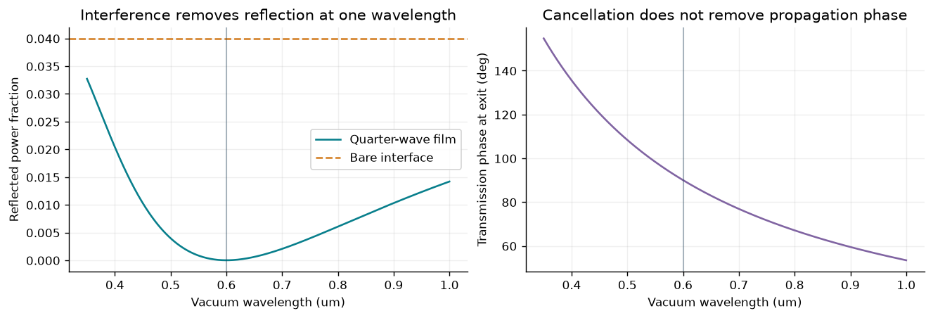
An exact normal-incidence, constant-index analytical film. Perfect antireflection at the design condition does not establish a real material’s broadband performance.
Moving a reference plane changes phase even in a uniform medium. If only the output plane moves a distance downstream, . This fact matters when comparing a zero-thickness sheet, a finite-height ridge, measured S parameters, and a stored training dataset.
2.9 Normalize a scattering matrix
For propagating ports with real positive admittance, scale each incoming/outgoing tangential field by . The resulting amplitudes have squared magnitude equal to normal power flux. Write
A lossless complete scattering description requires . A passive one requires for every input. Reciprocity and mirror symmetry are separate properties; a substrate can break the latter without breaking the former.
For our bare interface between two propagating channels,
The opposite reflection signs follow our field bases and port arrangement. is symmetric and unitary. Raw electric-field transmission coefficients from opposite sides need not be equal; their power-normalized counterparts are equal here. An evanescent solution with zero normal flux cannot be normalized as an independent unit-power propagating port by dividing by .
2.10 Give a sheet a current
Consider an ideal, local, purely electric surface at normal incidence. Let its sheet admittance be in siemens, and define the dimensionless quantity . Because there is no magnetic surface current, tangential electric continuity still gives . The electric jump condition adds a shunt current:
Solving yields
Here and at normal incidence. For , the sheet is passive and . The absorbed power follows directly from , rather than from unexplained missing channels.
This is also an equivalent-circuit language: the wave regions are transmission-line ports and is a shunt at their junction. Under , a capacitance per square has and an inductance has . Positive conductance dissipates power. An engineering convention using reverses these reactive signs.
For equal air ports and real ,
with equality at . A larger conductance eventually reflects more strongly instead of absorbing more. This 50% limit belongs to this one-sided, purely electric, equal-medium sheet model. A backed sheet, added magnetic response, different environment, or different illumination changes the problem.
2.11 Retrieve only what is identifiable
For the equal-air electric shunt at the common sheet plane,
Before applying it, check the complex continuity relation , the reference planes, the exterior impedances, and the model assumptions. Near , small errors in can produce large parameter errors; at this inversion is undefined. A passive model should also satisfy the appropriate energy constraints.
An arbitrary finite film or patterned ridge does not automatically meet those conditions. In particular, entrance and exit planes of a finite layer are different planes. Deembedding removes known propagation phases; it does not prove that the remaining response is a local electric shunt. A successful fit at one frequency is not a validation over wavelengths, angles, polarizations, or geometries that were not checked.
The Chapter 1 model introduced two effective response channels. Its balanced electric-like/magnetic-like construction is richer than a pure electric shunt, which enforces and cannot independently specify an arbitrary transmission amplitude and phase. General susceptibility-tensor retrieval and bianisotropic sheet synthesis require more unknowns, illuminations, and consistency conditions than the scalar illustration here.
2.12 Where did the missing light go?
Return to the air-surrounded sheet with . One incident beam gives , , and . Now illuminate it coherently from both sides, with total incoming power normalized to one:
Adding the outgoing field contributions before calculating their powers gives
At , every outgoing amplitude vanishes: the ideal model absorbs all the incoming power. At , the electric field at the sheet is a node and absorption vanishes. The material parameter has not changed. The incident coherent state has changed, so its overlap with the dissipative scattering channel has changed.
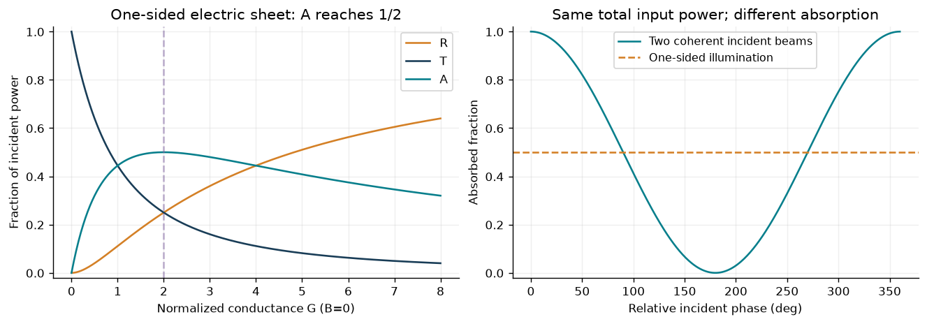
The one-sided and two-sided experiments have different incident states and the same explicit power normalization. Perfect two-sided absorption here requires exact sheet parameters and coherent excitation at the stated reference planes; it is not a fabricated-device result.
This is an entry point to coherent perfect absorption, a research topic developed by Chong, Ge, Cao, and Stone. Our shunt derivation illustrates a restricted analytical example and does not reproduce their slab calculation. An experiment would additionally need controlled phase, matched spatial modes, calibrated power, material dispersion/loss, and uncertainty.
2.13 Carry this into the next chapters
Before accepting any metasurface response, ask:
Which field basis, time convention, and reference planes define its complex coefficients?
Which admittance or channel normalization converts those coefficients to power?
Which waves propagate, which decay, and which are at cutoff?
Which boundary currents or geometry support the proposed transformation?
Does the model conserve or dissipate power appropriately for every relevant illumination?
Which independent condition would test the claimed retrieval or design?
Chapter 3 adds patterned geometry and a full-wave library; Chapter 4 adds diffraction channels; Chapter 5 assembles transformations. Chapter 10 uses data that must preserve exactly these conventions. Continue with the nine worked examples, computational lab, and self-check and mini-project.
For an independent foundational route, the Cornell ECE 3030 handouts cover plane waves, polarization, interfaces, and multilayers. MIT’s optics lecture notes provide complementary wave and polarization material. The explanations, derivations, figures, and experiments in this chapter are original course material.
Linked computational investigations
Continue with ms-09: spectral bandwidth, ms-10: independent cells versus supercells, and ms-11: bounded optimization with independent checks. These executed studies use the same explicit ridge geometry and connect spectral response, model approximation and design validation. The inverse-design study is a direct full-wave baseline for later AI comparisons.