Question: which simple calculation would expose a wrong sign, a wrong normalization, or an unsupported physical interpretation?
These examples accompany the chapter, browser/notebook lab, and self-check. They use , spatial , peak electric amplitudes, and positive real nonmagnetic bulk indices. Predict the sign or limiting behavior before reading each calculation.
1. Find the magnetic-field sign
A plane wave propagates along positive in air, with electric phasor . Maxwell’s relation gives
Thus points along positive , as required. Reverse the wavevector while keeping electric polarization along the same direction: the magnetic field reverses, and the power flux points along negative .
Check: an implementation using the same electric-to-magnetic sign for both propagation directions will give the wrong boundary equation. This is the physical origin of rather than .
2. Can a passive interface give t = 1.2?
At normal incidence from glass to air ,
The powers are
There is no gain: the electric field has a different power weighting in the two media. Reversing the illumination gives and , but the transmitted power remains 0.96. The power-normalized transmission amplitude is in either direction.
Prediction to retain: a field coefficient and a power-normalized S parameter can be different numbers without disagreeing physically.
3. Make only one polarization reflectionless
For air to glass,
At this angle, and . The TM admittances agree:
Therefore . For TE,
This calculation uses the common tangential-electric basis. A conventional reflected -unit-vector coefficient may have the opposite sign from our TM coefficient, while its zero and power agree. Brewster matching is a polarization-specific condition, rather than a universal reflectionless interface.
4. A field beyond total reflection
Take glass to air at and . The critical angle is , so transmission is evanescent. Here
For TE,
The transmitted amplitude is nonzero, yet because . Meanwhile . Its amplitude decay length is
At , the electric amplitude is reduced by ; intensity is reduced by . There is no distant transmitted beam in this semi-infinite lossless problem. Another interface within the decay region would define a different experiment.
5. Turn a line into a circle
Start with . Apply the ideal retarder :
At a fixed , its physical field has and . Its tip moves from positive toward positive . The norm stays one because .
For a linear analyzer at any angle ,
An analyzer therefore gives the same transmitted intensity for every angle, even though the incident field vector rotates in time. A global phase applied to both Jones components changes neither the polarization ellipse nor this intensity; a relative phase can change the ellipse.
6. Add material to remove reflection
Match air to glass at with an ideal constant-index film:
Then , , and the numerator of the film reflection coefficient is . Thus and . The transmitted electric coefficient at the film exit is
Zero reflection does not imply unit electric amplitude or zero transmission phase. The phase above includes propagation from the entrance reference to the exit reference. The cancellation is exact for the stated ideal design condition; real dispersion and fabrication errors need their own study.
7. The reference plane
At one common plane in air, an absent sheet has , so the electric-shunt retrieval gives . Now leave the incident reference fixed and move the output plane downstream by . The measured transmission becomes through propagation alone.
Blindly inserting it into the same-plane shunt formula produces
The apparent negative conductance would falsely suggest an active sheet in empty space. The continuity check already rejects this data interpretation: . Removing the known propagation factor restores . Deembedding is necessary here; it is not, by itself, evidence that an arbitrary finite structure is a local sheet.
8. Read a shunt and its uncertainty
For equal air ports and ,
Inverting recovers . In contrast, a purely reactive gives , , and with . Reactive current changes scattering and stores/releases energy without net cycle-averaged dissipation in this ideal model.
For the inverse relation , the sensitivity is
Thus a fixed absolute uncertainty in the measured complex field can cause a large absolute parameter error near a transmission zero. At exactly zero the inverse is undefined. Good retrieval retains complex and , verifies at the same plane, checks passivity, and tests another independent illumination or frequency before making a broader claim.
The notebook now makes this sensitivity test directly editable. Its controlled perturbation changes both coefficients consistently with the synthetic shunt relation; a separate printed continuity residual shows why independent measurement errors need their own model test. Compare the exact finite error with the derivative estimate, and report the ratio of perturbation magnitude to transmission. The approximation requires that ratio to be much smaller than one.
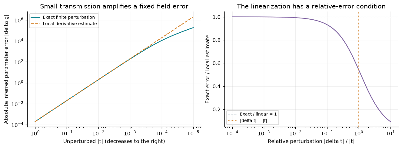
Original deterministic sensitivity calculation from the analytical sheet inverse. A small absolute field error becomes a large parameter error near zero transmission. The local estimate loses validity when the perturbation is comparable to transmission; these are synthetic model-consistent perturbations, not measured uncertainty.
9. Absorb two beams with their phase
Keep and illuminate coherently from both sides with . The input power is one. Multiplying by the equal-air scattering matrix gives
Then
Equal phase gives ; opposite phase gives ; a phase difference of gives . The one-sided 50% bound has not been violated under its original assumptions: we changed the illumination. Add fields at each outgoing port before squaring, rather than adding the two separate one-sided power results and discarding interference.
This is an exact analytical prediction for the specified sheet and coherent inputs. Experiments would additionally need spatial-mode matching, phase control, calibration, and a material implementation. For the broader research context, see Chong et al. on coherent perfect absorption.
A teaching sequence
Use Examples 1–2 as a ten-minute diagnostic before introducing a numerical solver. Use 3–4 to test polarization and complex wavevectors; 5–6 to connect phase to observable changes; 7–8 to critique a retrieval; and 9 as a capstone prediction. Two moving arrows on paper can illustrate the outgoing complex-field sums before any calculation.
Continue with the lab, then try the self-check and mini-project. The numerical notebook and browser are tools for checking a prediction, not substitutes for stating its assumptions.