Central question: how do we turn a desired outgoing wave into a physical design and evidence that it works?
Chapter 4 identifies the channels a periodic structure can support. Chapter 3 computes how a repeated unit cell responds. Synthesis connects a desired field to geometry, then tests the assembled structure. A target phase profile is a useful starting point; its realization must also satisfy amplitude, polarization, power, and fabrication constraints.
We develop a complete teaching example: a six-cell dielectric beam deflector, selected from periodic-cell data and verified as a full-wave supercell. We then introduce focusing with a scalar aperture model and polarization control with analytical Jones matrices. The worked examples, computational lab, beam-steering notebook, and wavefront-model notebook preserve their separate evidence levels.

This saved expanded design has h = 1.80 µm and L = 6Λ = 3.90 µm. All six ridges are solved together, and the entire sequence repeats. The case controls update widths and height together with the diffraction powers. Focusing and Jones examples later in this chapter are separate models.
5.1 Outcomes and the synthesis chain
By completing the chapter, you should be able to:
Derive beam-steering and focusing phase profiles under stated wave conventions.
Explain spatial sampling, phase quantization, and incomplete library coverage.
Select geometries using circular phase errors and power constraints.
Distinguish a local-cell prediction from a full-wave assembled structure.
Report incident-normalized target power and conditional diffraction purity separately.
Analyze a scalar line focus and define its numerical metrics honestly.
Derive geometric phase in an explicitly defined circular basis.
The working sequence is target field → representation → realizable response → geometry → independent verification. At each arrow, retain the assumptions being introduced. Prerequisites are the Chapter 4 channel conventions, Chapter 3 complex responses, Fourier series, and basic linear algebra.
| Model | Question answered | Evidence supplied here |
|---|---|---|
| Ideal continuous mask | What spatial field would produce the desired wave? | Analytical phase profiles |
| Sampled/local mask | What does discretization and a unit-cell library predict? | Exact staircase coefficients and selected responses |
| Periodic full-wave structure | What do the coupled ridges actually scatter? | Converged TE supercell order powers |
| Scalar finite aperture | How does a prescribed finite field propagate? | Line-focus profiles and window/grid checks |
| Analytical Jones matrix | How does a stated anisotropic response transform polarization? | Geometric phase and conversion fractions |
5.2 Specify a target field before choosing a phase
At a reference plane, a scalar target can be written
For vector fields, specify two complex polarization components, or an appropriate Jones transformation. Also state wavelength, illumination, exterior media, reference planes, aperture, and the desired observable. A beam direction, target-order power, focal width, and polarization-conversion fraction are different objectives.
For time dependence and an incident factor , a multiplicative phase contributes a local transverse wavevector
Thus a constant gradient gives
This is a wavefront-momentum relation. A realizable structure still needs a scattering calculation for its amplitudes. The generalized-refraction work of Yu and colleagues is a foundational reference; use Chapter 4 for the discrete orders of an actually periodic geometry.
For a periodic ramp increasing by over , and the intended outgoing order is . A noninteger accumulated ramp does not become an arbitrary new Floquet order when the geometry is forced to repeat; the repeated pattern has its own Fourier spectrum.
5.3 A phase gradient does not set efficiency
For one TE plane wave, normal power flux is proportional to . If all incident power were transmitted into one desired wave with no reflection or other channels, its electric-field ratio would have to satisfy
A unit-amplitude phase-only field does not generally have that flux. Complete passive scattering must account for impedances, all outgoing channels, and the local/collective response. The work on perfect reflection/refraction by Asadchy and colleagues develops the physical constraints beyond prescribing a phase gradient.
One synthesis route starts directly from the boundary fields. For a surface normal directed from region 1 to region 2,
These equivalent electric and magnetic surface currents describe the field jumps. Turning them into a realizable sheet requires a constitutive response consistent with passivity, reciprocity where applicable, and sufficient information about both illuminations/polarizations. This chapter’s implemented route instead selects dielectric geometries from a library and verifies their full scattering; it does not retrieve a general bianisotropic susceptibility tensor.
5.4 Spatial sampling and phase quantization
Divide one period into intervals of pitch . Assign a complex value to interval , whose center is . The exact Fourier coefficient of this staircase field is
The sinc factor represents each finite-width interval. A discrete sum without this factor describes a different source model. For ideal samples ,
For six levels this coefficient fraction is about 0.9119. It is a property of the scalar staircase field, not a full-wave device efficiency. Physical order powers additionally require flux normalization and a consistent scattering solution.
A sufficient local sampling condition for a phase-only target is , which avoids exceeding the phase-gradient Nyquist limit. This alone does not exclude additional physical diffraction channels or prove that a local-response approximation is accurate. Use the actual primitive/supercell period and exterior light cones as well.
5.5 Build a realizable phase library
The original Chapter 3 library fixes and spans about over widths 0.08–. It cannot represent a complete ramp accurately. We keep that library intact and create a new Chapter 5 dataset.
The notebook screens five declared common heights, from 0.60 to , over the same width domain. The coarse phase span first exceeds a full cycle at . At that height, it computes 161 widths and checks each at versus 32. A continuous unwrapped span exceeding does not by itself guarantee complete usable coverage after applying a transmission threshold.
For each desired sample phase , retain accepted rows with and minimize circular error:
The global offset is free for the ideal beam direction but changes the selected geometries. We search 361 fixed offsets, minimizing mean squared phase error using unit-cell data only. The expanded library matches all six sample phases within in the saved run. The supercell results are evaluated afterward; they are not used to select the offset or height.
This is a small, transparent discrete synthesis procedure. It is separate from gradient-based geometry optimization, generative design, or surrogate-assisted search. The exported records preserve both successful and limited-library designs.
5.6 Verify the complete beam-deflector geometry
The reference has six centered ridges per supercell, each with pitch , so . The wavelength is , with ridge/gap indices 2.4/1, incident index 1, substrate index 1.5, and normal TE incidence. All ridges within a sequence share one height.
The desired transmitted order has
Reflection supports , while transmission supports . Each channel receives its own complex coefficient and power normalization. This geometry and illumination differ from the six-post COMSOL example cited in Chapter 4.
For the full-wave model, the Chapter 3 TE Fourier equations are extended to all six coplanar rectangles. Their exact permittivity coefficients are
The complete Maxwell boundary problem is solved at the common top and bottom faces. All retained Fourier harmonics interact through this material matrix. Face-referenced decaying propagation factors avoid growing evanescent transfer factors.
For the local comparison, a staircase made from the individual cell coefficients gives estimated order powers , and an analogous reflected estimate. These are model predictions. Their total need not equal one, because the interfaces and differing neighbors were not solved collectively.
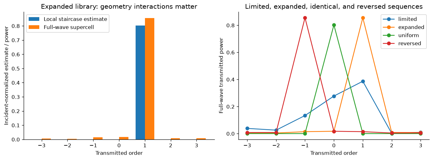
The local-cell design is tested against the full repeated geometry. Identical cells suppress nonzero supercell amplitudes; reversing a sequence reverses the order-power distribution.
The expanded design directs about 85.54% of incident power into . Its total transmission is about 91.14%, so the desired order contains about 93.85% of transmitted power. Report the denominator: these two percentages describe different observables. The local staircase estimate of target-order power is about 80.27%.
The original limited library gives about 38.62% incident-normalized power in for its selected sequence. It is retained as an informative constrained design, not omitted because its performance is lower. Six identical ridges have zero nonzero-order amplitudes to numerical accuracy, even though those directions are allowed. Reversing the expanded sequence puts the dominant transmitted power in .
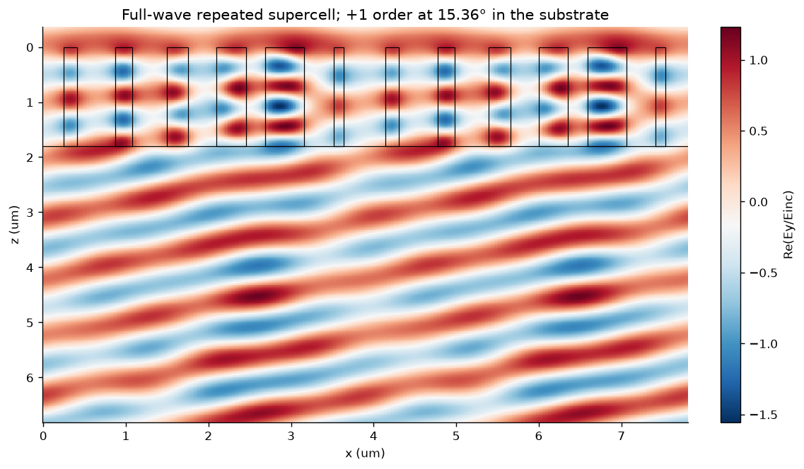
Full-wave field reconstruction of an infinitely repeated TE supercell. Order-resolved modal powers, rather than the field image alone, establish the far-field fractions.
5.7 Validate synthesis at more than one level
The final four supercells are compared at and 192, corresponding to 289 and 385 harmonics. Every reported open-order power and meaningful complex transmission coefficient is checked. The largest saved power change is below and the largest open transmitted-amplitude change below . All-channel power balance is checked separately.
Increasing the number of cells while retaining the same integer reduces the represented physical Fourier bandwidth. For identical-cell embedding, the audit scales the supercell truncation with the number of primitive cells, compares with the primitive calculation, and verifies the forbidden supercell amplitudes. A mirror-reversed sequence must exchange positive and negative order powers under this normal-incidence, mirror-related geometry.
Three supercells are also compared at matching with the separately developed grcwa implementation. Its cell-averaged raster is refined from 512 to 4096 samples. The fine-raster order-power and zeroth-order complex-transmission differences are below in the saved audit. Both implementations use RCWA; FEM/FDTD and experiment remain distinct future comparisons.
5.8 Synthesize a focusing wavefront
For normal incidence and a focus at in a homogeneous output medium, equal accumulated phase gives
For a point focus in two transverse dimensions, replace with . At oblique incidence subtract the incident tangential phase as well. The paraxial limit is ; the exact profile avoids that approximation in the target path length, while a scalar aperture model still has its own limits.
The executed example uses a cylindrical line focus: 48 pitch-wide cells, aperture , design distance , wavelength , and output index 1.5. It compares a continuous ideal aperture, a sampled phase aperture, and an aperture assigned the expanded library’s complex local coefficients.
Scalar angular-spectrum propagation is
with positive imaginary square roots for forward evanescent decay. The FFT assumes a periodic computational window, so pad the aperture and refine window size and spatial spacing independently. An exact sampled plane wave checks propagation phase. These are checks of the scalar model, not a full-wave finite-lens validation.
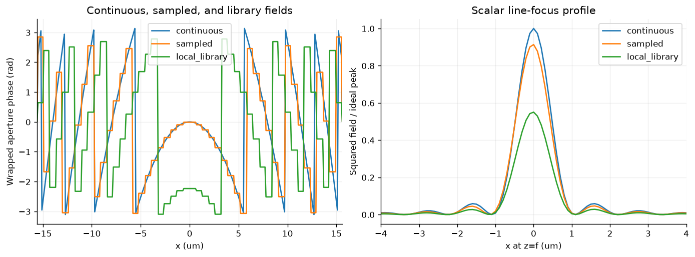
The library aperture includes local amplitude and phase, including its selected global phase offset. That offset does not change the propagated intensity, so the plotted absolute phases need not coincide. Scalar propagation is an approximation to a possible finite device and has no full-wave focusing-efficiency claim.
At the design plane, the saved continuous profile has FWHM about , and the local-library model about . The notebook also reports peak squared field relative to the continuous reference and the fraction of modeled line intensity in a stated window. Those are scalar line metrics, not a physical focusing-power efficiency or two-dimensional encircled energy. A finite aperture can shift the axial intensity maximum away from the design distance.
5.9 Amplitude control and polarization
A single width generally changes amplitude and phase together. Synthesis of an arbitrary complex field may require additional independent geometric parameters, anisotropy, interference, multiple layers, or a more constrained target. An amplitude taper can change scalar sidelobes and peak/width tradeoffs; its physical implementation must also account for discarded, reflected, and converted power.
For an anisotropic element with principal coefficients , rotated by in the laboratory plane,
Define the fixed-basis circular states . Then
The converted component acquires geometric phase . Its amplitude is controlled by . For an ideal lossless retarder, and , so the conversion fraction is . A half-wave response maximizes conversion; a rotation angle by itself does not establish high efficiency.
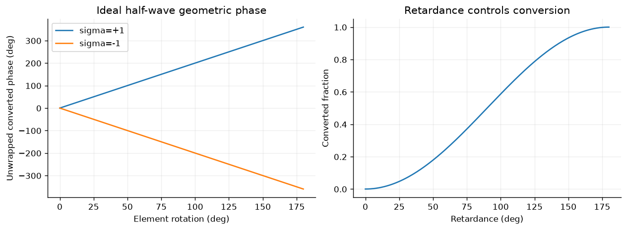
An ideal analytical Jones model. These curves are separate from the scalar TE ridge calculation and require a vector unit-cell design for physical realization.
The notebook verifies these coefficients, unitary half-wave matrices, and conversion fractions. For a physical anisotropic metasurface, extract a complete, consistently normalized vector response and retain the unwanted polarization channel. Arbabi and colleagues provide a primary example of dielectric phase/polarization control.
5.10 Objectives, constraints, and research extensions
An optimization objective can penalize complex-response mismatch, undesired orders, and fabrication sensitivity. For example, combine a target-order reward with a penalty on unwanted transmitted/reflected powers, subject to allowed widths, gaps, heights, material properties, and passivity. State the illumination and weighting of wavelengths/angles before optimization. Preserve independent verification conditions rather than selecting them after seeing the best result.
The implemented calculation uses discrete phase matching and a global-offset grid. It does not execute a full geometry optimizer, hologram reconstruction, robust tolerance study, or active learning. Those are useful lab/project extensions connecting to Chapters 6 and 10. A broadband claim additionally requires material dispersion and wavelength-dependent scattering, not only recalculating a monochromatic phase formula.
5.11 Exercises
Derive the sign of the target order for a positive phase ramp under our convention. Predict the result after spatial reversal.
Derive the TE amplitude required for complete transmission into an oblique wave. Explain why direction alone cannot specify power.
Integrate the staircase Fourier coefficient and recover the sinc factor. Separate its coefficient fraction from physical diffraction efficiency.
Compare phase-offset selection using RMS phase error and a complex-amplitude objective. Verify changed geometries independently.
Explain the local-mask power imbalance without interpreting it as physical absorption in a lossless structure.
Scale the harmonic bandwidth when changing supercell length. Design a convergence study that preserves physical resolution.
Derive the focusing phase for oblique illumination or an off-axis focus. Define an observable appropriate to a scalar line focus.
Derive the circular-basis Jones coefficients and identify the converted and unconverted channels.
Propose a finite-device, FEM/FDTD, dispersion, or fabrication test with a measurable acceptance criterion.
Continue with the worked examples and computational lab. The published source bundle preserves code, data, requirements, and validation so students can extend a specific stage through a pull request.
Linked computational investigations
Continue with ms-09: spectral bandwidth, ms-10: independent cells versus supercells, and ms-11: bounded optimization with independent checks. These executed studies use the same explicit ridge geometry and connect spectral response, model approximation and design validation. The inverse-design study is a direct full-wave baseline for later AI comparisons.