Central question: how can a patterned interface change a wave, and what evidence tells us what it actually does?
Imagine illuminating a thin patterned surface with a plane wave. Some power returns, some continues, and the outgoing fields can have different phases, directions, or polarizations. A design must specify which of these changes is desired and how success will be measured. A striking field image or a phase plot alone does not answer every part of that question.
This chapter introduces the computational language used throughout the course. We begin with geometry and wave intuition, then use an explicitly ideal sheet model to explore amplitude, phase, interference, and conservation. The worked examples, first computational lab, and executed notebook turn the ideas into predictions that can be checked and edited.
1.1 Learning goals and preparation
After this chapter, you should be able to:
Describe a metasurface as a structured electromagnetic scattering interface.
Distinguish an element, a primitive period, a supercell, and a finite aperture.
Interpret a complex response coefficient and separate amplitude, phase, and power.
Explain how electric and magnetic responses can contribute to directional interference.
State the assumptions behind a sheet, local-cell, or full-wave model.
Frame a design question with a measurable objective, constraints, and validation.
Useful preparation is familiarity with sinusoidal waves, complex numbers, electromagnetic fields, and basic energy conservation. Python experience is helpful for editing the notebook, but the browser explorer needs no installation. Chapter 2 will develop electromagnetic boundary conditions, normalization, polarization, and sheet descriptions more systematically.
1.2 What is a metasurface?
A metasurface is a laterally structured interface or array designed to produce a specified electromagnetic response. Its repeated or varying building blocks are often called meta-atoms, although they are engineered structures rather than literal atoms. Examples include printed microwave conductors, apertures, dielectric ridges, and optical nanoposts.
Many implementations use subwavelength lateral features and a thickness small compared with a conventional wavefront-shaping component. There is no universal thickness or pitch threshold that alone establishes a useful metasurface model. Some dielectric structures have appreciable propagation through their height, and a spatially varying sequence can have a much larger repeat than its element spacing.
The response depends on geometry, material properties, illumination, and interactions between elements. A single geometric parameter rarely specifies an arbitrary complex transformation for every wavelength, angle, and polarization.
| Description | Useful viewpoint | A limitation to check |
|---|---|---|
| Bulk metamaterial | Effective propagation through a structured volume | Whether a bulk effective description is justified |
| Metasurface / structured interface | Engineered scattering and field transformation near an interface | Whether a local sheet or cell model captures the actual structure |
| Diffraction grating | Periodic structure and its outgoing diffraction channels | Which orders carry power and how strongly |
| Conventional phase element | Optical path or impedance variation across an aperture | Thickness, bandwidth, and sampling constraints |
These viewpoints overlap. A periodic metasurface diffracts according to the same channel physics as a grating. Calling a structure a metasurface does not remove unwanted diffraction, coupling, or material loss. The flat-optics overview by Yu and Capasso provides context for engineered interfaces and wavefront control.
Microwave frequency-selective surfaces, transmitarrays, and reflectarrays provide part of the engineering context for optical flat components. The operating band changes materials, fabrication, loss, dispersion, and measurement methods; a geometric scaling alone need not preserve performance. The Yu–Capasso review connects those traditions without implying that one design transfers unchanged between them.
| Intended function | What to specify and measure |
|---|---|
| Beam steering or splitting | Power in each desired direction/order, angular response, and polarization |
| Focusing or imaging | Wavelength, aperture, focal region, spot/line width, and collection normalization |
| Polarization transformation | Desired output polarization, conversion power, and leakage |
| Spectral filtering or absorption | Band, transmitted/reflected channels, loss, and bandwidth |
| Reconfigurable communication surface | State-dependent response plus the actual illumination and system channel |
A passive surface need not be lossless. A tunable surface changes state under external control; tuning alone does not establish electromagnetic amplification or nonreciprocity. A scalar coefficient describes one selected polarization channel, while a general polarization transformation requires multiple coupled field components. Arbabi and colleagues demonstrate phase/polarization control with a specific dielectric-post platform; its reported results are not predictions of our scalar model.
1.3 Identify the scales before choosing a model
For free-space wavelength , positive real refractive index , and frequency ,
Compare dimensions with the wavelength in the relevant medium, not only with . State the illumination angle and polarization as well; they change the scattering problem.
Element: one chosen building block, with dimensions such as width and height.
Pitch: spacing between neighboring element sites.
Primitive period: the smallest translation restoring the complete material pattern.
Supercell: a computational or physical sequence containing multiple sites, possibly with different elements.
Aperture: the finite illuminated or fabricated extent, whose edges affect the outgoing field.
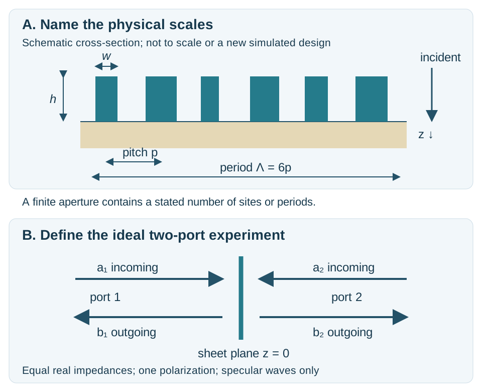
Original schematic of two descriptions. The upper drawing names physical scales; the lower drawing defines the ideal two-port experiment. No fitted relation between their geometry and channel strengths is assumed. An aperture can contain many periods.
For six different sites spaced by , a repeated sequence has period . Six identical sites can preserve the smaller primitive period. The available supercell labels and their actual amplitudes are different questions. Chapter 4 derives the channels; Chapter 5 verifies both sequences with a full-wave calculation.
Subwavelength pitch alone does not guarantee that a varied supercell has only a zeroth diffraction order. Nor does it prove that each cell behaves independently of its neighbors.
1.4 A complex number describes more than a phase
We use the phasor convention
The magnitude and phase describe the field relative to a reference. A reflection or transmission coefficient is a complex ratio of an outgoing field amplitude to the chosen incident amplitude. Its phase also depends on where the reference planes are placed.
A coefficient has field magnitude 0.8 and phase . In equal-impedance media at normal incidence, its transmitted power fraction is . At an interface with different impedances or oblique incidence, the correct flux factors must be included. Chapter 2 will develop those factors; the present model deliberately keeps the exterior impedances equal.
At , the phase is undefined. Near zero amplitude, a phase can be numerically unstable and physically unhelpful for a transmitted-wave design. Keep magnitude or power beside every phase plot, and state the threshold used when reporting phase.
The wrapped phase lies on a circle. and differ by a circular separation of , not . An unwrapped phase follows a continuous branch across a parameter sweep; it still needs meaningful nonzero amplitude and sufficiently fine sampling.
1.5 How elements respond and interfere
An incident field drives charge, current, and polarization in a structure. An electric-dipole-like response is associated with oscillating electric charge separation. A magnetic-dipole-like response can arise from circulating currents or displacement-current patterns; it does not require a naturally magnetic material at the operating frequency.
The resulting fields interfere with one another and with the incident wave. Suitable electric and magnetic contributions can cancel in one direction and reinforce in another. The dielectric Huygens-surface work of Decker and colleagues develops this physical idea for specific dielectric structures. Reproducing a paper’s device performance requires its geometry, materials, illumination, and numerical or experimental evidence.
Several design mechanisms are useful:
| Mechanism | Main control | Tradeoff or condition |
|---|---|---|
| Resonant response | Geometry/material-dependent resonance | Phase and amplitude vary with frequency and loss |
| Propagation phase | Optical path or guided propagation through an element | Height, index, modal coupling, and dispersion matter |
| Geometric phase | Orientation of an anisotropic response | Depends on polarization channel and conversion amplitude |
| Collective/nonlocal response | Interaction across several elements | A local independent-cell description may fail |
These mechanisms can coexist. A response library from repeated identical cells includes that repeated environment. Assembling different cells changes the environment and requires an additional test. Chapter 3 builds a library, while Chapter 5 compares its local prediction with the complete repeated structure.
1.6 Start with a transparent analytical model
To separate response reasoning from geometry and solver setup, define a two-port sheet. Port 1 and port 2 represent the specular waves on opposite sides, in equal-impedance media. For a reciprocal, mirror-symmetric response,
The incident amplitudes are and the outgoing amplitudes , all referenced to the ideal sheet. One-sided incidence sets . Losslessness for arbitrary incoming fields requires , which is stronger than checking only .
Use two unit-magnitude channel functions, and :
The even/odd eigenvalues of are and . The transparent limit gives . The labels electric-like and magnetic-like are effective channel coordinates in this teaching model; their numerical values are not retrieved electric or magnetic dipole moments.
For each channel, choose the dimensionless ratio and strength :
For , the rational expression remains finite at resonance. When , define explicitly, including at . With real frequency and these parameters, , so the complete scattering matrix is unitary. The notebook verifies this algebra numerically and checks an independent electric-only shunt expression.
This model is deliberately restricted. It has no assigned width, height, material dataset, diffraction, polarization conversion, or absorption. Its value is to make interference and physical consistency inspectable before adding geometry.
1.7 Predict four limiting cases
| Case | Parameters / condition | Prediction |
|---|---|---|
| Transparent | Both strengths zero | , |
| Electric-like only | Magnetic-like strength zero | Strong reflection at its resonance; transmitted phase undefined when |
| Balanced pair | Identical two channel functions | , , with unit transmitted power and varying phase |
| Detuned pair | Different resonance frequencies | Cancellation generally breaks; reflection and transmission redistribute power |
At the reference , the free-space wavelength is about . The electric-only preset has . The balanced preset has : zero reflected power and a transmission phase of relative to the transparent reference.
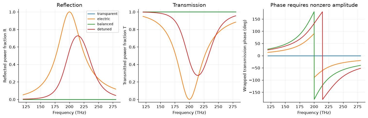
Power and phase describe complementary parts of the response. The electric-only transmission phase is masked at its exact zero. Perfect balanced matching is imposed by this ideal model.
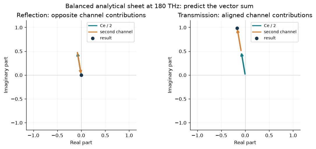
Original complex-plane illustration of the model’s channel contributions. These arrows are not separately retrieved dipole radiation fields.
Matching the channels over an entire frequency interval is an imposed idealization. Unit transmission in this model does not establish a practical, lossless, broadband Huygens surface or a geometry providing every desired phase.
1.8 Frequency dependence and bandwidth
The same surface is illuminated at many possible frequencies, but its response at those frequencies is linked by its physical dynamics and material properties. A monochromatic phase choice does not specify an independent response everywhere else.
For a meaningful continuous transmission phase, group delay is
The notebook compares two balanced ideal channels: a narrower phase transition has a larger peak delay. This illustrates spectral dispersion while preserving the model’s imposed unit transmission. It is not an achromatic metalens or a retrieved material group delay. Chapter 5 discusses focusing models, and later investigations will need justified material dispersion and wavelength-dependent geometry verification.
1.9 Choose evidence appropriate to the claim
| Evidence | What it can establish | What still needs checking |
|---|---|---|
| Analytical model | Behavior under explicit equations and assumptions | Whether those assumptions describe a physical geometry |
| Local unit-cell approximation | A response assigned from repeated-cell data | Differing neighbors, supercells, and aperture edges |
| Full-wave simulation | Maxwell scattering for the specified numerical model | Convergence, materials, illumination, and experimental relevance |
| Experiment | Performance of a measured sample in a stated setup | Calibration, uncertainty, repeatability, and collection geometry |
A simulation is not automatically converged because it finishes, and a model is not accurate merely because it conserves power. Record the source/version, parameters, conventions, numerical controls, checks, and scope. Chapter 6 develops these habits systematically; the existing full-wave chapters already apply them.
In a simple lossless two-port problem, . In a real diffracting or polarization-converting structure, include all relevant outgoing channels before attributing missing measured power to absorption. Finite collection angles and unmeasured polarization channels can also matter.
Applications require specific observables. Beam steering needs a target-order fraction and angular response. A lens needs a defined focal region, power normalization, width, and collection geometry. A polarization device needs desired conversion and leakage. A communication surface also needs system-level illumination and channel assumptions. A high phase span by itself is not a complete performance metric.
1.10 Formulate your first design question
Write an experiment specification before choosing a solver or an AI model:
Excitation: wavelength/frequency, incident medium, angle, polarization, and beam/aperture.
Target: desired complex field or measurable performance quantity, with its denominator.
Design space: geometry, materials, tunable states, and constraints.
Model: analytical sheet, local library, periodic full-wave structure, or finite device.
Evidence: limiting cases, numerical refinements, independent comparisons, and uncertainty appropriate to that model.
For example: “At normal incidence and one stated wavelength, select a dielectric sequence maximizing incident-normalized power in transmitted order +1, subject to width/gap limits, then verify all-channel scattering and convergence.” This is a testable objective. “Provide a full phase range with high efficiency” still needs wavelength, geometry, normalization, and acceptance criteria.
1.11 Course map and exercises
Chapter 2 establishes waves, boundaries, polarization, and power normalization. Chapter 3 computes unit-cell amplitudes; Chapter 4 develops periodic channels; Chapter 5 synthesizes and verifies wavefront transformations. Chapter 6 develops numerical methods. Chapters 7–9 have syllabus outlines for tuning, applications, and experimental/material considerations, and Chapter 10 develops AI workflows with independent verification.
Draw an element, primitive cell, supercell, and aperture for a proposed surface. State which dimensions you would compare with which wavelength.
Explain why a periodic metasurface can also be described as a diffraction grating. Identify a case where pitch and full period differ.
Compare , , and . Which have identical transmitted power in this model? Which have a meaningful transmission phase?
Use a pair of complex arrows to predict reflected cancellation and transmitted addition for the balanced model.
Derive the eigenvalues of the two-port scattering matrix and verify the transparent limit.
State which assumptions would fail for a substrate, oblique illumination, absorption, or polarization conversion.
Critique a claimed efficiency: identify the denominator, measured/simulated channels, material assumptions, and validation.
Propose one experiment connecting the analytical model to a specific full-wave geometry without assuming a parameter-to-geometry mapping.
Continue with the six worked examples and the first computational investigation. The browser explorer opens in a new tab; the source ZIP provides editable code, notebook, data, and validation.
Finish with the self-check answers, mini-project, rubric, and glossary. The worked guide also checks power normalization against a saved Chapter 3 full-wave result, making the evidence difference explicit before Chapter 2.