Central question: which beams can leave a periodic metasurface, and what calculation tells us how much power they carry?
Imagine six different elements spaced by . Repeat that six-element sequence and illuminate it at a free-space wavelength of . Can the surface scatter into a nonzero angle in air? Make a prediction before choosing a formula: does the relevant period equal the element spacing or the length of the complete repeated sequence?
This chapter develops the translation symmetry, the allowed wavevectors, and the numerical checks needed to answer that question. The browser explorer and editable notebook calculate channel geometry. The lab also specifies a later full-wave calculation for the channel amplitudes.
4.1 Goals and conventions
After this chapter, you should be able to:
Identify a primitive period and distinguish it from an element pitch or computational supercell.
Derive the Bloch phase and the tangential wavevectors of Floquet orders.
Classify each order separately in the reflection and transmission media, including grazing cutoff.
Explain why an allowed channel can have zero amplitude and why closed orders still matter numerically.
Set up a periodic scattering calculation and assess its order-resolved power and convergence.
Prerequisites are plane waves, phasors, tangential boundary conditions, Fourier series, and basic complex algebra. The worked examples and teaching guide include a short learning path.
We use time dependence and spatial dependence . The surface is near , periodic along with period , and invariant along in the introductory model. A plane wave arrives from and travels toward positive . Angles are signed from the relevant outward surface normal, with a positive angle having positive .
The incident and transmitted half-spaces are homogeneous, isotropic, lossless media with positive real indices and . We set initially. Materials inside a future scattering structure may be more complicated; the real-index channel tests below apply to its homogeneous exterior regions.
| Symbol | Meaning |
|---|---|
| , | Free-space wavelength and wavenumber |
| , | Structural period and reciprocal-lattice spacing |
| Incident tangential wavevector | |
| Diffraction-order label under our sign convention | |
| Index of the output region being examined: for reflection or for transmission |
4.2 Find the pattern that actually repeats
A translation by a primitive period restores the complete material distribution. Translating by one pitch in a row of different pillars generally replaces one geometry with another. Translating by the complete sequence restores it. For six distinct elements separated by , a possible primitive period is .
The word possible matters: if the sequence itself has a smaller repeating subset, use that smaller period. A numerical cell may contain several primitive cells for convenience, but its extra order labels do not create new physical scattering mechanisms.
For example, place six identical elements inside a computational cell of length . The structure still has period . In an expansion using , the smaller translation symmetry forces nonzero coefficients to occur only at supercell orders . Other supercell channels may lie inside the output light cone but have zero amplitude.
4.3 Translation symmetry and the Bloch phase
For one incident plane wave, the driven scattering solution lies in the same Bloch sector as the excitation. A field component can be written
It follows that
This is a phase relation between paired lateral boundaries. At normal incidence the multiplier is one. At oblique incidence, an ordinary zero-phase periodic condition generally represents a different excitation.
The boundary mapping direction matters. If a solver defines destination from source , the multiplier under our convention is . Reversing the mapping requires its inverse. Some solvers use a different phasor or built-in phase convention. Verify the actual translated plane wave instead of copying a sign from a screenshot.
Bloch wavevectors differing by a reciprocal vector
Replacing by leaves the translation multiplier unchanged because . This is the origin of reciprocal-lattice equivalence. It relabels harmonics; it does not change their physical tangential wavevectors when the labels are shifted consistently. The incident wavevector remains fixed by the physical incidence condition.
4.4 Derive the Floquet orders
Expand the periodic factor in a Fourier series:
Substituting gives
All harmonics have the same Bloch multiplier. The periodic pattern permits tangential momentum changes in integer multiples of . Material properties and boundary conditions determine the coefficients .
The following dimensionless form makes the design parameters easier to compare:
In a wavevector diagram, the orders are equally spaced points along the tangential axis. Changing incidence translates the whole set; changing changes its spacing.
4.5 Open, grazing, and evanescent channels
In output region , the homogeneous-medium dispersion relation gives
For an outward distance measured away from the surface, define
with the outgoing branch: nonnegative real for propagation and positive imaginary for decay. In laboratory coordinates, transmitted waves have and reflected waves have because their outward directions differ.
| Condition | Classification | Interpretation |
|---|---|---|
| $ | q_m | <n_o$ |
| $ | q_m | =n_o$ |
| $ | q_m | >n_o$ |
For an open order,
Do not clip an arbitrary value outside and report a grazing beam. First classify the channel. The notebook uses a dimensionless tolerance around and reports near-cutoff cases separately. That tolerance handles floating-point classification; it is not an uncertainty estimate for wavelength, material data, or geometry.
What does an evanescent order do?
If with , its amplitude varies as . Its amplitude decay length is ; its intensity decay length is . In the specified lossless homogeneous exterior, one such isolated outgoing harmonic carries no net normal time-averaged power. It can still store reactive energy, affect interface matching, and mediate coupling near the structure.
Consequently, “closed in the far field” does not mean “safe to remove from an RCWA expansion.” Near cutoff, can be small and the decay length large. Numerical harmonic convergence and port/reference-plane placement deserve particular attention there.
Count every potentially open order
The strict interval for an open integer order is
The endpoints must be tested separately for grazing. The notebook enumerates a conservative enclosing integer interval and adds closed neighbors for plotting. A fixed window such as can silently miss channels when the period or output index increases.
4.6 Two output media, two channel maps
Apply the classification separately with for reflection and for transmission. Both sides share , but their light-cone boundaries differ. A larger refractive index can support additional propagating orders.
For , , and normal incidence, air supports . An output medium with supports . At oblique incidence, the set can become asymmetric: negative and positive order labels need not open together.
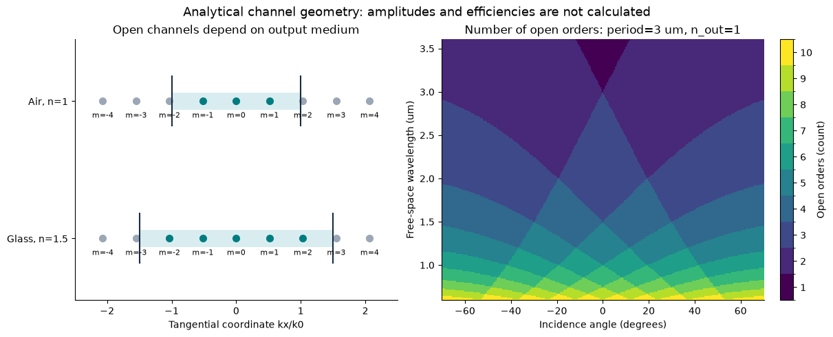
Figure 1:Analytical channel geometry from the executed notebook. The map counts possible outgoing channels. No scattering amplitude or diffraction efficiency is assigned to them.
4.7 Channel existence and diffraction efficiency
Knowing and identifies the available basis waves. Solving Maxwell’s boundary-value problem determines their amplitudes. A symmetry-forbidden order, an unpatterned interface, or destructive interference can give zero amplitude in an open channel.
To convert amplitudes into power, state their normalization. For a TE wave represented by in an isotropic lossless medium,
For an open transmitted order with ,
With equal permeabilities, the factor is . This expression is for the stated TE electric-field amplitude. A TM coefficient defined using tangential needs a different admittance factor; using gives a corresponding expression with in place of . For compatible power-normalized port amplitudes, squared magnitude directly gives the power fraction.
For a passive scattering problem, use all outgoing propagating channels and any genuine absorption:
At exact grazing, a bounded field amplitude has zero normal flux. Power normalization becomes delicate as the normal component approaches zero. A closed-channel field coefficient should not be counted as an extra far-field power fraction.
An analytical amplitude benchmark
At a flat nonmagnetic interface, translational invariance permits only the physical specular response, even if an artificial periodic cell lists many open channels. At normal incidence from to , the TE Fresnel amplitudes are and . Thus , , and . Squaring alone would incorrectly report .
The notebook checks this case and a total-internal-reflection limit. These are analytical interface checks, not simulations of a patterned metasurface. For numerical mode/flux normalization examples, see the official Meep mode-decomposition tutorial.
4.8 Finite arrays and grating lobes
An infinite periodic calculation produces discrete Floquet directions. A finite illuminated array has angular lobes with nonzero width. For equally spaced prescribed scalar sources with identical weights and the incident phase progression, a normalized array factor is
Its maxima occur at the same tangential matching conditions when they lie inside the output light cone. Increasing narrows the peaks. The notebook computes the sum directly, avoiding a removable singularity in a sine-ratio formula.
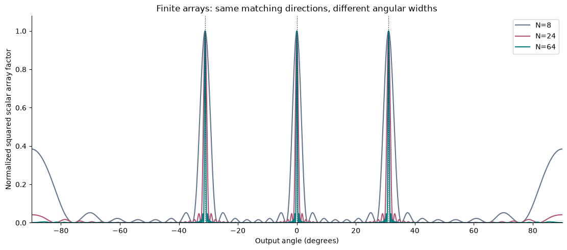
Figure 2:Prescribed scalar array factors for 8, 24, and 64 repeated sources. The vertical markers are analytical Floquet directions. This plot does not include an element radiation pattern, mutual coupling, vector boundary matching, or a power-normalized metasurface efficiency.
In scanning-array language, unwanted additional visible maxima are grating lobes. Suppose all incidence angles satisfy and the zeroth order remains open. A sufficient condition to keep every nonzero order closed throughout that scan is
For equal unit indices and the limiting full scan toward , this becomes the familiar strict half-wavelength-spacing condition. At normal incidence alone the corresponding bound is . Always state the medium, wavelength, scan range, and whether equality means an excluded grazing case. For a broadband requirement, check the smallest relevant wavelength and the actual dispersion.
4.9 Phase gradients and generalized refraction
For a prescribed transmission phase , tangential phase matching motivates
This connects to the generalized reflection/refraction formulation of Yu et al.. It specifies a desired phase-matching relation; useful efficiency also requires an electromagnetic design that supplies the required amplitudes and boundary response.
If the complex transmission function is periodic over and makes an ideal integer phase winding , then the average gradient is . With our Fourier convention, an ideal prescribed factor shifts the transmitted tangential wavevector to order . A sampled or imperfect phase profile generally has additional Fourier harmonics.
A real sequence of resonant elements need not realize that ideal scalar transmission function. Material dispersion, amplitude variation, coupling, and impedance mismatch can change its performance. Floquet channels describe the periodic scattering basis; a phase-gradient design seeks to excite selected coefficients in that basis.
4.10 From a channel map to a periodic solver
Start with a homogeneous or flat-interface cell whose response is analytically known. Then introduce a simple grating. Use the following checks before a large parameter sweep:
Specify coordinates, the actual period, excitation, exterior indices, polarization, and phasor convention.
Apply the correct lateral Bloch phase and check that a translated incident wave satisfies it.
Use homogeneous exterior regions and outgoing ports or suitable absorbing boundaries. Include every propagating order across the complete sweep on both sides.
Match solver order labels to tangential wavevectors; a solver may index orders with a different sign or basis.
Normalize incident and outgoing power consistently. Compare modal power with an independent flux calculation where available.
Refine mesh, harmonic truncation, port distance, or domain/PML settings as appropriate. Power balance alone cannot establish convergence of each order’s amplitude or phase.
Record reference planes, complex coefficients, failures, and the residual in all-channel power accounting.
The full-wave lab outline gives a staged flat-interface, dielectric-grating, and optional six-pillar investigation. The official COMSOL beam-deflector example provides a concrete six-post Si/SiO2 reference using periodic boundaries and diffraction-order ports. Its supplied geometry and solver instructions are external reference material; our executed results here are analytical.
Beyond the introductory model
For a two-dimensional lattice,
In an isotropic lossless exterior, compare its squared magnitude with . The notebook includes a small rectangular-lattice example so that the one-dimensional condition is not mistaken for a general two-dimensional rule. Lossy, anisotropic, nonlocal, or time-modulated systems require an appropriate dispersion relation and outgoing-wave/energy-flow analysis. A real-angle arcsin test is not a universal classification algorithm.
4.11 Exercises and discussion
Derive the Bloch multiplier for a translation by . Explain why the multiplier alone cannot identify the incident diffraction-order label.
Solve the six-element opening puzzle for air and for an output index of 1.5. Calculate each open angle.
Using , , and in air, calculate the phase advance and every open order. Which sign of the first order propagates?
Find the incidence angle where reaches grazing for , , , and . Repeat for .
Explain how a computational supercell can list propagating channels that have zero amplitude because the actual primitive period is smaller.
Derive the TE power factor and explain how the definition of a TM field coefficient changes the normalization.
Compare finite arrays of different lengths. Which features are determined by periodicity, which by aperture length, and which are absent from the scalar model?
Design a numerical convergence study near a diffraction cutoff. Distinguish a channel-classification tolerance from a solver convergence tolerance.
Propose a full-wave experiment that separates an incorrect period, incorrect Bloch phase, omitted output channel, and poor phase-gradient design.
Continue with the worked examples, browser explorer and lab, and executed notebook.
References and further reading
Yu et al., Light Propagation with Phase Discontinuities: Generalized Laws of Reflection and Refraction, Science 334, 333-337 (2011). Article; author’s publication page.
COMSOL, Diffraction Grating Theory. A software reference for grating directions; distinguish ray-direction models from full-wave amplitude calculations.
COMSOL, Metasurface Beam Deflector, Application ID 115971. A periodic six-post reference geometry and solver example.
Meep, Mode Decomposition. Official diffraction and modal-power examples for a future solver implementation.
The derivations, figures, exercises, and exploratory code in this chapter are original course material. The browser and notebook models state their assumptions explicitly so that their claims can be extended through later full-wave validation.
- Yu, N., Genevet, P., Kats, M. A., Aieta, F., Tetienne, J.-P., Capasso, F., & Gaburro, Z. (2011). Light Propagation with Phase Discontinuities: Generalized Laws of Reflection and Refraction. Science, 334(6054), 333–337. 10.1126/science.1210713