Central question: how can a geometry become a trustworthy entry in a metasurface design library?
Suppose a design calls for a transmitted phase of and at least 80% transmitted power. A width sweep produces many colorful phase values. Which geometry should you choose? Before choosing, establish what field was normalized, where its phase was measured, which outgoing channels were included, and whether increasing numerical resolution changes the answer.
This computational chapter builds that chain of evidence. It follows the Floquet conventions of Chapter 4, then calculates the amplitudes those channels carry. The worked examples, lab and browser explorer, and executed notebook share one original Python solver and one exported dataset.

The reference width is 0.325 µm; the library sweeps w while keeping period, height and materials fixed. The ridges extend indefinitely along y and repeat along x. Purple dashed lines identify one unit cell. The lab drawing updates with the selected width.
3.1 Outcomes and prerequisites
After completing the investigation, you should be able to:
Specify geometry, materials, illumination, periodicity, and reference planes unambiguously.
Extract complex reflection/transmission and convert field amplitudes into power.
Explain a Fourier-modal unit-cell calculation and its numerical truncation.
Distinguish algebraic residuals, conservation checks, and numerical convergence.
Export a versioned response library and select a geometry with explicit feasibility criteria.
Identify when a periodic-cell prediction needs a supercell or finite-device test.
Prerequisites are Maxwell boundary conditions, phasors, Fresnel coefficients, Fourier series, eigenvectors, and basic Python. Reading Sections 4.1–4.7 first provides the channel geometry. Chapter 1 and Chapter 2 supply the earlier foundation.
3.2 Define the electromagnetic experiment
A unit cell describes a structure repeated indefinitely under a specified Bloch excitation. Its response includes interactions with that repeated environment. When every ridge width changes, the entire periodic environment changes along with it.
The reference cell has a ridge centered at , width , height , period , and invariance along . The layer occupies . Air lies above it at and a homogeneous substrate below at . Illumination travels toward positive .
| Quantity | Reference value | Role |
|---|---|---|
| Repeat along | ||
| 0.08– | Swept ridge width, 50 samples | |
| Fixed patterned-layer thickness | ||
| Free-space wavelength | ||
| , | 2.4, 1.0 | Ridge and gap indices |
| , | 1.0, 1.5 | Incident medium and substrate |
| Reference incidence | ||
| Polarization | TE, , | Scalar Maxwell reduction |
All indices are positive, real, constant, and nonmagnetic. They define an ideal dielectric model without assigning measured material properties. A research library should use a stated dispersion model and measured or otherwise justified optical constants.
We use and . The incident equals one at ; reflected coefficients are referenced to and transmitted coefficients to . Keeping these two reference faces fixed makes the width comparison meaningful.
3.3 Choose a solver that matches the structure
| Method | Natural use | Numerical controls to vary |
|---|---|---|
| Fourier modal / RCWA | Laterally periodic structures represented as uniform layers along the propagation direction | Fourier harmonics; geometric/material representation; layer slicing for a varying vertical profile |
| Finite elements | Complex shapes, material interfaces, frequency-domain fields | Mesh, polynomial order, exterior boundaries/ports |
| FDTD | Broadband time-domain response and spatially resolved fields | Spatial grid, run time/decay, PML, source/monitor placement |
The course implementation is a restricted RCWA calculation: one rectangular patterned layer with exact Fourier coefficients. Its vertical eigenmode propagation is analytic, so there is no finite-difference mesh or staircased height to refine. The main truncation is the number of spatial harmonics. A sloped sidewall or vertically varying cell would need additional layers or another solver.
The Meep grating and mode-decomposition tutorials provide a useful later FDTD comparison, including flux normalization and phase references. The grcwa documentation describes the separate RCWA implementation used in our numerical audit. Solver conventions must be mapped before comparing signs and amplitudes.
3.4 Channels, complex amplitudes, and power
For retained integer orders , define
The outgoing root has nonnegative real and imaginary parts. A positive real gives a propagating channel; a positive imaginary gives outward decay. At exact cutoff , this implementation requests a parameter perturbation rather than using a singular grazing basis.
The exterior expansions are
For these electric-field TE amplitudes, the order powers relative to incident normal flux are
Closed exterior orders have zero normal outgoing power in these lossless half-spaces. Sum every open order to obtain and . For this lossless model, to numerical accuracy. With absorption in a more general solver, the missing fraction requires a consistent dissipated-power calculation.
At the library reference parameters, , exceeding both exterior indices. Only is open, so and . If period, wavelength, or angle changes, enumerate the channels again. A zeroth-order library becomes incomplete when other orders open.
For an open zeroth-order channel, the power-normalized coefficient is . Record whether a solver exports this quantity or an electric-field ratio. Reciprocity comparisons require compatible normalization, channel directions, reference planes, and the appropriate reversal of transverse wavevectors.
3.5 Derive the restricted TE Fourier model
For a nonmagnetic scalar permittivity and ,
Write and expand as a Fourier series. Projection onto the retained harmonics gives
For a centered rectangle with fill fraction ,
These coefficients are analytic, including the limit. There is no pixel grid in the course solver. The matrix is Hermitian for these real-index materials, and its eigenproblem is
The square roots in again use nonnegative real/imaginary branches. The derivative-mode matrix is . To avoid exponentially growing transfer factors, define forward coefficients at the top face and backward coefficients at the bottom face:
Continuity of and its normal derivative, for common permeability, yields
Here and are diagonal exterior matrices and excites order zero. Recover
The code implements these equations in solve_cell. Its sample_ey function reconstructs fields inside and outside the ridge layer. film_reference supplies a separate scalar Fresnel/Fabry-Perot benchmark. See Moharam and Gaylord’s foundational formulation for the broader RCWA method.
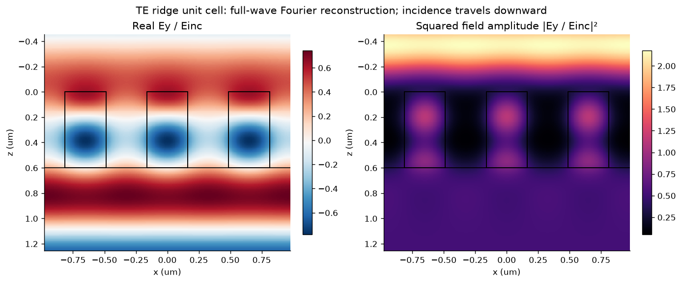
Original full-wave field reconstruction for the central cell. Outgoing evanescent harmonics contribute to the near field. The squared field amplitude is distinct from power and energy density.
3.6 Extract phase at stated reference planes
A phase is meaningful relative to an excitation and a plane. Suppose an incident monitor is above the ridge and an output monitor below it. If both measured ratios use incident at , then
Removing these homogeneous propagation phases returns the two face-referenced coefficients. The notebook tests this algebra with synthesized monitor offsets; the RCWA calculation itself matches directly at the two interfaces.
The wrapped phase jumps at . For a smooth parameter sweep, phase unwrapping can reveal the continuous path. The path can be misleading near , where phase is poorly defined and numerical noise becomes dominant. Keep amplitude beside every phase plot and use a stated amplitude/power threshold for design.
For comparing a response with a desired phase, use the circular difference
The direct subtraction gives , while their circular separation is . For a change in height, even a bare homogeneous propagation path changes phase. Define a common physical comparison plane or a clearly stated background reference before attributing that change entirely to the ridge response.
3.7 Validate before exporting
Three questions require separate evidence:
| Question | Check | Limitation |
|---|---|---|
| Was the truncated linear system solved? | Relative algebraic residual | Does not assess harmonic truncation |
| Is power accounted for? | All-channel $ | 1-R-T |
| Does numerical refinement change the response? | Complex-amplitude, power, and meaningful phase changes with | Agreement of finite truncations is an empirical test, not a rigorous error bound |
The reference investigation passes 18 analytical interface/uniform-film cases. At normal incidence with , it returns , , , and . A larger artificial period gives additional open labels with zero amplitudes at that flat interface.
For every width, the library compares with : 49 versus 65 harmonics. It requires , changes in and below , a circular phase change below , and power residual below 10-8. The saved run’s worst is about . Six additional points are checked at .
The audit also tests reflected/transmitted order sets at oblique incidence, mirror-related order powers, input guards, and reconstructed field continuity. Eight cases are compared against grcwa at matching harmonic count, while its independent raster representation is refined from 256 to 2048 samples. At the fine raster, the largest complex zeroth-order transmission difference is below . Both codes use RCWA; a comparison using FEM/FDTD and any experimental validation remain future work.
The notebook’s spectral-neighborhood plot provides an exploratory illustration at fixed harmonic order. Its wavelengths are outside the exported single-wavelength library domain and require their own convergence studies before library acceptance.
3.8 Build a response library a colleague can reuse
A useful record preserves more than width and phase:
Experiment: geometry, units, material model, wavelength, angle, polarization, and primitive period.
Response: complex amplitudes, order labels, total and order-resolved powers where necessary, and phase reference planes.
Evidence: solver/source version, environment, numerical controls, refinement changes, residuals, and acceptance thresholds.
Scope: supported parameter domain, excluded physics, and known incomplete design coverage.
The reference JSON combines this metadata with the 50 rows; its CSV is convenient for plotting and later model fitting. The width in each row overrides the illustrative central width in the metadata. Preserve different experiments as versioned datasets rather than merging rows with incompatible references.
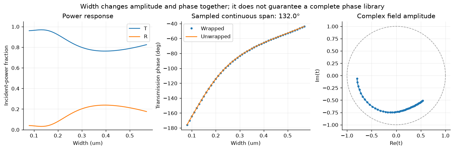
The computed width sweep spans about continuously. This height and width range do not provide complete coverage, even before imposing a minimum transmission requirement.
3.9 Select a geometry with a feasibility test
For this first design exercise, retain accepted rows with and minimize the absolute circular phase error. A request is feasible only when that error is at most .
The saved library supplies a width near for a target of , with and phase error about . A target of remains unmet under the same criteria; the closest eligible row misses by about . Report this result directly. Expanding the height range, changing the geometry, or revising the objective would define a subsequent design investigation.
Interpolating a response library requires additional checks. Interpolate real/imaginary parts or another representation respecting phase periodicity; verify new geometries with the solver, especially near rapid response changes. For Chapter 10, separate geometry groups before splitting data and retain numerical uncertainties. Fifty related samples at one wavelength are a teaching dataset, with no claim about general AI performance.
3.10 From a periodic library to a real device
A local-periodicity approximation assigns a cell the response it would have in an infinite array of identical neighbors. A wavefront-shaping device places different geometries next to one another. Their coupling and collective diffraction can alter the response.
Before claiming device efficiency, assemble an appropriate supercell or finite structure, include its actual outgoing channels, and compare its scattering with the library-based prediction. Sharp gradients, resonant near fields, aperture edges, and rapidly changing neighboring geometries deserve particular attention. An element library is an input to that test, rather than a completed beam-deflector simulation.
For a research cell, add physical material dispersion, relevant loss, geometric tolerances, and solver checks appropriate to the chosen fabrication geometry. Chapter 4 supplies channel bookkeeping; Chapter 5 develops synthesis, and Chapter 6 develops numerical validation.
3.11 Exercises
Specify the smallest set of metadata that makes a complex transmission coefficient reproducible. Explain why a phase value without reference planes is incomplete.
Derive the TE power factors from the normal component of the time-averaged Poynting vector.
Derive the rectangle Fourier coefficients, including and . What changes when the ridge is translated laterally?
Explain why can conserve power while disagreeing with a higher-order calculation. Distinguish exterior propagating channels from retained internal Fourier harmonics.
Use the notebook to change . Reassess phase coverage, transmission, and convergence; define how you will compare phases between different heights.
Repeat an oblique-incidence calculation. Enumerate open orders in both media and retain all their powers.
Compare two interpolations near a wrapped-phase jump. Verify a proposed intermediate width with a new Maxwell solve.
Define a multi-parameter library for Chapter 10, including grouped data splits and numerical-uncertainty records.
Design a supercell comparison that tests the local-periodicity approximation. State an observable and acceptance threshold before running it.
Continue with the six worked examples and computational lab. Download source and data there to extend the calculation through a pull request.
Linked computational investigations
Continue with ms-09: spectral bandwidth, ms-10: independent cells versus supercells, and ms-11: bounded optimization with independent checks. These executed studies use the same explicit ridge geometry and connect spectral response, model approximation and design validation. The inverse-design study is a direct full-wave baseline for later AI comparisons.
- Moharam, M. G., & Gaylord, T. K. (1981). Rigorous coupled-wave analysis of planar-grating diffraction. Journal of the Optical Society of America, 71(7), 811–818. 10.1364/JOSA.71.000811