Central question: when does a learned model help us design a metasurface, and what evidence makes its proposed design credible?
Imagine building a library of unit cells. For every geometry, you solve Maxwell’s equations over a frequency band and record complex reflection and transmission. A new specification arrives: a different phase, a broader band, or a different incidence angle. Can we reuse the library to search efficiently? Can we tell when the requested response lies outside what the library supports?
This chapter develops that workflow, from the electromagnetic problem to a learned approximation and back to electromagnetic verification. Start with the physical question; choose a learning method after defining the observable, constraints, and evidence you need.

The executed AI pilot uses an analytical sheet response with an abstract design coordinate. No nanostructure is assigned to that coordinate. This drawing explains the scattering model; a physical ridge or other geometry requires the separate full-wave dataset stages.
10.1 Learning goals and prerequisites
After this chapter, you should be able to:
Write forward prediction, inverse design, and optimization as distinct mathematical problems.
Build a dataset whose inputs, outputs, normalization, and split match the intended physical claim.
Compare a learned surrogate with a simple baseline on geometries withheld from training.
Explain why an accurate average prediction can still yield an unreliable optimized design.
Validate a candidate against physical constraints and an independent electromagnetic calculation.
You should be comfortable with complex amplitudes, S parameters, power balance, basic linear algebra, and numerical optimization. Start with the NumPy kernel notebook, then use the scikit-learn comparison notebook. The pilot guide gives a sequence and readiness checks. Use Chapters 2–4 for the wave, unit-cell, and diffraction prerequisites, Chapter 5 for synthesis, and Chapter 6 for the numerical verification needed before a full-wave dataset study.
10.2 Three problems that should be kept distinct
Let describe the design: lengths, widths, thicknesses, rotation angles, material choices, or a spatial pattern. Let describe the operating conditions: frequency, incident angle, polarization, temperature, or bias. Let be the response we want to predict or control.
The electromagnetic forward problem is
may be an analytical model, an RCWA calculation, a finite-element model, or an FDTD simulation. A learned surrogate approximates this mapping over a specified domain. The trainable parameters belong to the model; they are different from the design variables .
The inverse-design problem starts with a desired response and seeks one or more designs that produce it. One useful formulation is
measures the response mismatch, defines admissible designs, and penalizes an undesirable property such as sensitivity to fabrication errors. Hard constraints, such as a minimum feature size, should remain explicit even if penalties are also used.
A surrogate-assisted search replaces expensive calls to during candidate selection with calls to . The final candidate still needs evaluation with , and often with a more accurate calculation than the one used to generate the training library.
Early work by Peurifoy et al. illustrates learned forward scattering and inverse search for multilayer particles. That example motivates a computational approach; its performance does not establish accuracy for an unrelated unit-cell family.
10.3 Decide what the model must predict
For a single polarization and a simple two-port unit-cell calculation, useful outputs may include complex and . For polarization conversion, the output may be a Jones matrix. When several Floquet channels propagate, use the appropriate scattering matrix and preserve the mode ordering.
Intensity alone cannot recover phase. If an application needs wavefront control, training only on discards essential information. Conversely, optimizing phase while ignoring a near-zero amplitude can produce an unusable design.
Complex representations and phase wrapping
A convenient representation is
At multiple frequencies, concatenate these quantities in a documented order. A complex transmission loss can be written as
This expression equals the sum of squared real and imaginary errors. It avoids a discontinuity at a selected phase branch cut. An alternative is to represent phase with sine and cosine, together with a separate amplitude, while ensuring that the predicted sine/cosine pair is normalized when reconstructing phase.
Consider phases and . Their ordinary numerical difference is , but their smallest angular separation is . A circular error is
Report phase errors only where both amplitudes exceed a declared threshold. At a transmission zero, phase is undefined. Do not use a threshold to hide poor amplitude prediction: report amplitude errors and the fraction of excluded samples separately.
Power normalization matters
For power-normalized propagating modes, the squared magnitude of an S parameter is a power fraction for the corresponding incident mode. An electric-field transmission coefficient between unequal media generally needs an impedance or longitudinal-wavevector factor before it becomes transmitted power. Record the solver’s convention and reference planes. Never train on coefficients from incompatible normalizations without reconciling them.
10.4 Build a dataset that answers a physical question
Treat each simulation record as evidence with provenance. The following information belongs in the data description:
| Record | Why it matters |
|---|---|
| Geometry ID and dimensions with units | Identifies related spectra and permits reconstruction |
| Materials and dispersion model | The same geometry can have a different response with different material data |
| Frequency, angle, polarization, and port basis | Defines the excitation and output channels |
| Boundary conditions, mesh or harmonic order, and solver version | Makes the calculation reproducible |
| Complex response and normalization/reference planes | Preserves amplitude and phase meaning |
| Power balance and convergence evidence | Helps distinguish numerical artifacts from physical trends |
| Data split and provenance | Prevents accidental reuse of test examples during development |
Split according to the claim
Suppose each geometry contributes 101 frequency samples. If you shuffle all rows and split them at random, the same geometry can appear in training and test sets at nearby frequencies. That experiment can assess interpolation within observed geometries; it does not establish performance on unseen geometries.
For new-geometry prediction, assign complete geometries to training, validation, or test sets. Fit scalers and other preprocessing only on the training set. Use validation data to choose model settings. Reserve the test set for the final evaluation. These practices follow the general guidance on leakage and preprocessing in the scikit-learn documentation.
State the split’s intended difficulty. Randomly held-out geometries within a dense design region test interpolation. A withheld geometric interval, material family, or incidence range tests a different and often harder form of generalization. Report these results separately.
10.5 Start with a baseline you can understand
Before training a large network, try nearest-neighbor retrieval, interpolation, or a simple regression model. These baselines show how much information is already available in the library. Compare methods on the same split, input information, target representation, and error metrics.
Kernel regression
The starter notebook uses a Gaussian kernel to compare scalar design parameters:
For training inputs , define . If the rows of contain response spectra, kernel ridge regression solves
Solve the linear system rather than explicitly calculating a matrix inverse. The length scale controls smoothness across the design coordinate; regularizes the fit. We select both on the validation set. Complex outputs can be handled as complex columns here, equivalently using separate real and imaginary targets with the same real kernel. See the kernel ridge reference for the broader method.
A neural network replaces this kernel expansion with learned nonlinear transformations. A multilayer perceptron can accept a small parameter vector; a convolutional architecture may suit a pixelated geometry. Architecture alone does not determine performance. Training-data coverage, target choice, regularization, and the evaluation problem remain central.
A neural surrogate you can inspect
For the scalar design coordinate in our example, standardize the input using the training mean and standard deviation:
One hidden layer and a linear output layer give
Here is a learned feature vector, not an electromagnetic field. For frequencies, pack the output as . With hidden units, the matrices have shapes and . Biases add parameters. With and , the network has trainable parameters. The 40 training geometries still provide only 40 independently sampled spectra; 101 frequencies do not turn them into 4040 independent geometries.
A useful conceptual training objective combines response error and weight regularization:
Backpropagation applies the chain rule to compute derivatives of this loss with respect to weights and biases. The optimizer then updates them. During forward-model training, the design coordinates and reference spectra remain fixed. During an inverse search, the trained weights remain fixed and the candidate design changes. Keeping those two operations separate prevents a common conceptual error.
Software loss conventions matter. Averaging squared error over packed real coordinates gives half the mean squared complex error over frequencies. Libraries also normalize regularization differently. The conceptual above is therefore not a claim that two packages’ alpha parameters are interchangeable. The notebook selects models using a separately calculated complex RMSE.
Our MLP uses tanh hidden units, linear outputs, L2 regularization, and L-BFGS optimization. It standardizes inputs using training data and reports optimizer warnings. Feature scaling and initialization sensitivity are discussed in the scikit-learn neural-network guide; the MLPRegressor API documents the optimizer controls. A maximum-iteration warning means the requested stopping criterion has not been established. It must remain part of the reported evidence.
Make the comparison fair and interpretable
The executed comparison uses identical geometry IDs and spectra for nearest retrieval, complex linear interpolation, KRR, and an MLP. KRR has 12 validation candidates; the MLP has six. This is a comparison under declared small search budgets, not an equal-compute competition. Architecture and regularization are chosen on validation data using a fixed initialization. Two additional neural initializations are then evaluated without changing the configuration or selecting a lucky seed.
Linear interpolation is a particularly useful baseline for one smooth design coordinate. It brackets a query between training coordinates and blends their complex spectra. Outside that bracketed region the implementation clips to the closest endpoint and reports how many test coordinates fall outside the training range. Neither interpolation nor a neural network provides evidence for an untested material or geometry family.
Use several complementary metrics: complex-response RMSE, power-fraction error, maximum error over the band, and phase error above the amplitude threshold. Report results per geometry as well as an aggregate; a small average can conceal a failed narrow resonance.
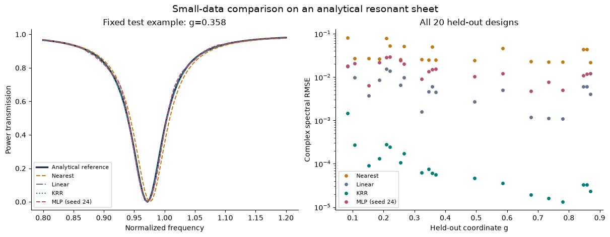
Figure 2:Saved output from the comparison notebook, using the declared 40/20/20 split. This is an analytical teaching experiment; its ranking does not establish a universal best model. The notebook contains the numerical tables, initialization results, and complete code.
In the published run, test complex RMSE is approximately 0.0414 for retrieval, 0.00800 for interpolation, 0.000353 for KRR, and 0.0165 for the primary MLP. The network improves on retrieval but does not beat the two smoother baselines on this task. Across its three initializations, MLP RMSE has mean 0.0232 and sample standard deviation 0.00732. This describes training variability on one fixed split, not a confidence interval for performance on other datasets. Three rejected validation configurations emit optimizer warnings; the selected configuration and its repeats finish without warnings. The notebook preserves all of that evidence.
10.6 Why inverse design is not simply the forward map reversed
Different geometries can produce nearly the same response. The inverse mapping may therefore be set-valued. An illustrative algebraic example is : for , both and are valid, but their average fails. A regression model trained to average conflicting inverse labels can therefore return a design that matches none of the valid solutions.
One remedy is to search through a forward surrogate. Another is a tandem network: an inverse model proposes a geometry, and a fixed, previously trained forward surrogate scores its response:
The forward model’s weights remain fixed while gradients update the inverse model. Liu et al. developed this approach to address non-unique inverse scattering examples. It shifts the training objective toward response consistency, but still inherits forward-model errors. Geometry bounds and manufacturing constraints must also be enforced.
Conditional generative models offer a further possibility: generate several candidate geometries for a target, then filter and verify them. Their diversity is useful only if candidates are feasible and their verified responses satisfy the task. A visually plausible pattern is not evidence of electromagnetic performance.
Optimization can exploit model errors
Consider a surrogate with small average error but an incorrectly predicted high-efficiency region near a data boundary. An optimizer may select precisely that region. Its search is not a random draw from the test distribution, so average test error can underestimate the risk at the chosen design.
Evaluate several promising candidates with the original model, inspect where the proposed design lies relative to the data, and refine the training set when appropriate. Keep the final test set independent of this adaptation. For costly solvers, active learning can select new simulations based on uncertainty or expected improvement, but compare the total number and cost of simulations with a conventional search.
10.7 Physical checks, uncertainty, and verification
For a passive device represented in a complete, compatible power-normalized propagating-port basis, the scattering matrix obeys
For a lossless device it becomes equality when all outgoing power channels are included. Reciprocity can impose in an appropriately paired modal basis. Do not impose these relations blindly on evanescent amplitudes, truncated channel sets, incompatible normalizations, or active/nonreciprocal systems.
These relations can be used as diagnostics, architectural constraints, or additional training penalties. Satisfying a penalty at a finite set of samples does not prove broadband causality or correctness for unseen geometries. A power-balanced model can still predict the wrong phase or resonance frequency.
Uncertainty estimates also require evaluation. An ensemble’s spread or a probabilistic model’s variance can be informative, but should be checked against held-out errors and domain shifts. Disagreement and confidence are not automatic guarantees. Distinguish uncertainty in the surrogate from uncertainty in geometry, material data, measurement, and the electromagnetic solver itself.
For a final design, report:
Its design vector, constraints, and operating conditions.
The surrogate prediction and the independently evaluated response on the same axes.
Mesh/harmonic/domain convergence and all-channel power accounting where applicable.
Sensitivity to fabrication and material variation.
Data-generation, training, search, and verification costs.
If generating the training data costs , then the total learning-assisted cost includes
Use measured costs appropriate to the actual solver and hardware. A fast prediction may be attractive for repeated design tasks while offering no overall saving for a single design.
10.8 Worked model: a synthetic resonant sheet
To practice the workflow without a commercial solver, consider a lossless symmetric two-port model with equal media, power-normalized amplitudes, and time dependence . Define normalized frequency , normalized linewidth , and detuning :
It follows directly that
At resonance, and . Far from resonance, transmission approaches unity. For the example, let a dimensionless design coordinate control
This mapping is deliberately synthetic: is not a documented pillar radius or fabricated geometry. The notebook samples entire spectra at different , fits a surrogate on one subset, chooses its settings on a validation subset, and evaluates held-out designs. It then searches for a target spectrum and checks the selected candidate against the exact formula.
For a symmetric two-port matrix , power balance for one incident port is only the diagonal part of . The off-diagonal condition is . Here is purely imaginary, so that condition also holds. The comparison notebook checks both identities. They apply to this model and its specified port basis.
Retrieving an exact training spectrum automatically preserves this model’s power balance, even when its resonance is in the wrong place for the requested design. Conversely, a regression can have very small complex error and a nonzero power residual. Accuracy and physical consistency answer different questions; report both.
Inspect physical consistency in the complex plane
For this reconstructed equal-air electric sheet, the signed quantity
vanishes on a circle centered at with radius . Its interior corresponds to a passive reconstructed response; its exterior would require gain under these specific assumptions. The comparison notebook plots the frozen predictions in this plane and reports the signed diagnostic over all held-out geometries.
Complex linear interpolation joins lossless training responses by chords inside that disk. It can therefore introduce artificial loss relative to the generator while preserving passivity. Nearest retrieval stays on the lossless circle even when the retrieved resonance is wrong. A small response error, passivity, and losslessness are distinct checks. Projecting onto the circle alone would not establish spectral accuracy, causality, or a realizable geometry.
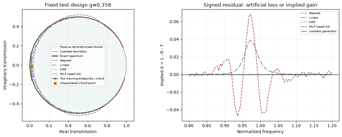
Original calculation from the frozen analytical comparison. The circle and interpolation chord expose artificial loss or implied gain in the reconstructed model. The signed quantity is a surrogate diagnostic, not measured material absorption; the notebook table also covers all held-out geometries.
That last step verifies the surrogate against its analytical data generator. It is not independent full-wave or experimental validation. The next lab stage replaces this generator with a converged unit-cell library while preserving the split, metrics, and reporting structure.
Continue with the Chapter 10 computational lab.
For the inverse comparison, retrieval returns an actual library design. Continuous surrogates search 901 coordinates separated by 0.001. A retrieval objective is flat between changes in the nearest neighbor, so attaching its winning spectrum to an arbitrary coordinate in that interval would be misleading. The notebook makes this distinction explicit and verifies every proposed coordinate with the analytical generator.
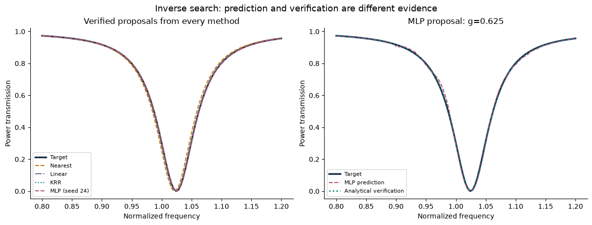
Figure 4:Inverse proposals from the comparison notebook. The target lies on the candidate grid, so some verified curves coincide exactly with it. The numerical table in the notebook distinguishes a small predicted mismatch from the actual mismatch after analytical verification.
10.9 Exercises and research discussion
Derive for the synthetic model. Explain why phase error is inappropriate at .
Construct two unit-magnitude complex coefficients at and . Compare ordinary phase subtraction, circular error, and complex-amplitude error.
Design two dataset splits: one for interpolation to new geometries and another for testing a withheld design interval. State exactly what each result would support.
A model predicts transmission with 1% mean power error. What additional evidence would you need before using it to design a metalens?
Explain how a tandem model can produce a small training loss and still propose an inaccurate design. Suggest a validation procedure.
Estimate the break-even number of repeated design tasks for a hypothetical library. Include data generation, failed simulations, retraining, and verification.
Propose a fabrication-robust objective such as expected response error plus a variance penalty. Explain how you would sample perturbations and evaluate worst cases separately.
Read one paper below and identify the design space, output representation, data generator, split, baseline, inverse objective, and independent verification. Which claims transfer to your proposed metasurface problem?
The pilot guide includes worked examples for conservation, phase wrapping, data leakage, inverse ambiguity, and computational cost. Use the remaining questions for discussion and independent reports.
References and further reading
Peurifoy et al., Nanophotonic particle simulation and inverse design using artificial neural networks, Science Advances 4, eaar4206 (2018). Article. A forward-surrogate and inverse-search example for multilayer particles.
Liu et al., Training Deep Neural Networks for the Inverse Design of Nanophotonic Structures, ACS Photonics 5, 1365-1369 (2018). Article; author preprint. Read for the non-uniqueness problem and tandem construction.
Malkiel et al., Plasmonic nanostructure design and characterization via Deep Learning, Light: Science & Applications 7, 60 (2018). Article. A case study connecting learned design/characterization to experiments.
Molesky et al., Inverse design in nanophotonics, Nature Photonics 12, 659-670 (2018). Review. Broader context for optimization beyond machine learning.
scikit-learn, Common pitfalls and recommended practices and Kernel ridge regression. Methodological references for data handling and the starter regression model.
These are foundational readings, not an exhaustive survey of current AI methods. The synthetic teaching model and exercises on this page are original course material.
Linked computational investigations
Continue with ms-09: spectral bandwidth, ms-10: independent cells versus supercells, and ms-11: bounded optimization with independent checks. These executed studies use the same explicit ridge geometry and connect spectral response, model approximation and design validation. The inverse-design study is a direct full-wave baseline for later AI comparisons.
- Peurifoy, J., Shen, Y., Jing, L., Yang, Y., Cano-Renteria, F., DeLacy, B. G., Joannopoulos, J. D., Tegmark, M., & Soljačić, M. (2018). Nanophotonic particle simulation and inverse design using artificial neural networks. Science Advances, 4(6). 10.1126/sciadv.aar4206
- Liu, D., Tan, Y., Khoram, E., & Yu, Z. (2018). Training Deep Neural Networks for the Inverse Design of Nanophotonic Structures. ACS Photonics, 5(4), 1365–1369. 10.1021/acsphotonics.7b01377
- Malkiel, I., Mrejen, M., Nagler, A., Arieli, U., Wolf, L., & Suchowski, H. (2018). Plasmonic nanostructure design and characterization via Deep Learning. Light: Science & Applications, 7(1). 10.1038/s41377-018-0060-7
- Molesky, S., Lin, Z., Piggott, A. Y., Jin, W., Vucković, J., & Rodriguez, A. W. (2018). Inverse design in nanophotonics. Nature Photonics, 12(11), 659–670. 10.1038/s41566-018-0246-9