دفترچهٔ فصل ۲: موجها، مرزها و ورقهها
اول پیشبینی کنید: آیا نسبت میدان ۰٫۸ میتواند ۹۶ درصد توان فرودی را عبور دهد؟ آیا میدان در محیطی با توان عمودی خالص صفر وجود دارد؟ آیا افزودن مرز بازتاب را حذف میکند؟ آیا فاز نسبی جذب را تغییر میدهد؟
این دفترچه با مدلهای تحلیلی دقیقِ تخت پاسخ میدهد. هندسهٔ فراسطح نقشدار را گسستهسازی نمیکند و حلگر تمامموج هندسهای ندارد. محیطهای حجمی ضریب شکست ثابت حقیقی مثبت دارند و غیرمغناطیسی و همسانگردند. رسانایی نامنفی ورقه میتواند توان تلف کند. قراردادهای و در سراسر دفترچه ثابتاند.
شناسهٔ موضوع: ms-01-waves-interfaces و مقدمات ms-03-sheet-response و ms-06-polarization.
متن توضیحی فارسی است؛ کد، جدولهای عددی، نمودارها و داده از مرجع مشترک انگلیسی میآیند. واژهنامه کلید خواندن برچسبها را دارد. این صفحه خروجی ذخیرهشده را نمایش میدهد؛ بستهٔ کامل قابل اجرا را از آزمایشگاه بگیرید.
from pathlib import Path
import sys,json,csv,hashlib,platform,html
import numpy as np
import matplotlib
import matplotlib.pyplot as plt
from IPython.display import display,HTML
ROOT=next((p for p in [Path.cwd(),*list(Path.cwd().parents)[:3]] if (p/'simulations/waves_interfaces.py').is_file()),None)
if ROOT is None:raise FileNotFoundError('Extract the complete Chapter 2 ZIP, preserving simulations/, notebooks/, and data/.')
sys.path.insert(0,str(ROOT/'simulations'))
from waves_interfaces import (interface,film,film_scattering,sheet,sheet_scattering,
                             coherent_sheet,retrieve_sheet,polarization,te_interface_fields,MODEL_VERSION)

# Editable reference experiment. Indices are ideal real constants, not measured dispersion.
N_INCIDENT=1.;N_OUTPUT=1.5;WAVELENGTH_UM=.6
N_FILM=np.sqrt(N_INCIDENT*N_OUTPUT)
THICKNESS_UM=WAVELENGTH_UM/(4*N_FILM)
FIELD_N1=1.5;FIELD_N2=1.;FIELD_ANGLE_DEG=50.
JONES_ALPHA_DEG=45.  # The plot compares relative phases 0, 45, and 90 degrees.
SHEET_G=2.;SHEET_B=0.
ANGLES_DEG=np.linspace(0.,85.,341)
DATA=ROOT/'data/chapter-02';DATA.mkdir(parents=True,exist_ok=True)
plt.rcParams.update({'figure.dpi':125,'font.size':10,'axes.spines.top':False,'axes.spines.right':False})
TEAL='#087f8c';ORANGE='#d48026';NAVY='#193d57';PURPLE='#8064a2'
def table(headers,rows):
    def esc(x):return html.escape(f'{x:.7g}' if isinstance(x,(float,np.floating)) else str(x))
    display(HTML('<table><thead><tr>'+''.join('<th>'+esc(x)+'</th>' for x in headers)+'</tr></thead><tbody>'+''.join('<tr>'+''.join('<td>'+esc(x)+'</td>' for x in row)+'</tr>' for row in rows)+'</tbody></table>'))
def ctext(z):return f'{complex(z).real:.5f}{complex(z).imag:+.5f}i'
table(['Parameter','Value'],[['n incident/output',f'{N_INCIDENT:g} / {N_OUTPUT:g}'],['Wavelength (um)',WAVELENGTH_UM],['Film index',N_FILM],['Film thickness (um)',THICKNESS_UM],['Time convention','exp(-i omega t)'],['Model version',MODEL_VERSION]])
print('Environment:',platform.python_version(),'NumPy',np.__version__,'Matplotlib',matplotlib.__version__)Environment: 3.12.1 NumPy 2.4.6 Matplotlib 3.11.1
۱. دامنه و توان
در برای ضرایب فرودی، بازتابی و عبوری از یک محور مشترک میدان الکتریکی مماسی استفاده کنید. پس در مرز دیالکتریک . ادمیتانس بیبُعد TE برابر و TM برابر است. ادمیتانس فیزیکی و دارای شاخهٔ خروجی یا میرا است.
علامت ضریب بازتابی TM با قراردادی که پایهٔ محلی را میچرخاند متفاوت است. در تابش عمودی هوا به شیشه، هر دو ضریب در پایهٔ مماسی و هستند و ، میدهند. پیش از رسم، صفر بروستر و زاویهٔ بحرانی شیشه به هوا را پیشبینی کنید.
theta_b=float(np.rad2deg(np.arctan(N_OUTPUT/N_INCIDENT)))
theta_c=float(np.rad2deg(np.arcsin(FIELD_N2/FIELD_N1))) if FIELD_N1>FIELD_N2 else None
interface_cases=[];angular={}
for name,n1,n2,angle,pol in [('normal TE',N_INCIDENT,N_OUTPUT,0.,'TE'),('normal TM',N_INCIDENT,N_OUTPUT,0.,'TM'),('Brewster TM',N_INCIDENT,N_OUTPUT,theta_b,'TM'),('TIR TE',FIELD_N1,FIELD_N2,FIELD_ANGLE_DEG,'TE'),('TIR TM',FIELD_N1,FIELD_N2,FIELD_ANGLE_DEG,'TM')]:
    v=interface(n1,n2,angle,pol)
    interface_cases.append(dict(name=name,parameters=dict(n1=n1,n2=n2,angle_deg=angle,polarization=pol),response=v))
table(['Case','r (tangential E)','t (tangential E)','R','T','Regime'],[[c['name'],ctext(c['response']['r']),ctext(c['response']['t']),float(c['response']['R']),float(c['response']['T']),str(c['response']['regime'])] for c in interface_cases])
fig,axes=plt.subplots(1,2,figsize=(11,3.8),layout='constrained')
for ax,name,n1,n2 in [(axes[0],'air_to_glass',N_INCIDENT,N_OUTPUT),(axes[1],'glass_to_air',FIELD_N1,FIELD_N2)]:
    for pol,color in [('TE',TEAL),('TM',ORANGE)]:
        v=interface(n1,n2,ANGLES_DEG,pol);angular[name+'_'+pol]=v
        ax.plot(ANGLES_DEG,v['R'],color=color,label=pol+' R')
        ax.plot(ANGLES_DEG,v['T'],'--',color=color,label=pol+' T')
    ax.set(xlabel='Incident angle (deg)',ylabel='Normal power / incident power',ylim=(-.02,1.04))
    ax.grid(alpha=.2);ax.legend(ncol=2,fontsize=9)
axes[0].set_title('A field ratio is not a power fraction')
axes[0].axvline(theta_b,color=NAVY,lw=1,alpha=.5);axes[0].text(theta_b-2,.48,'Brewster',rotation=90,ha='right')
axes[1].set_title('At critical angle, the outgoing channel closes')
if theta_c is not None:axes[1].axvspan(theta_c,85,color=TEAL,alpha=.08);axes[1].axvline(theta_c,color=NAVY,lw=1,alpha=.5)
plt.show()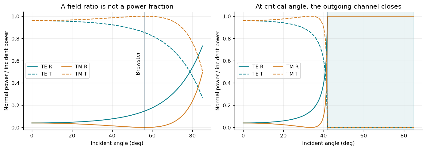
۲. میدان اوانسنت
برای شیشه به هوا بالاتر از زاویهٔ بحرانی، و . میدان ناصفر، کانال انتشار توان عمودی نیست. و را بازسازی و را مستقیم محاسبه میکنیم.
در آستانهٔ دقیق قطع، TE دارای مماسی و TM دارای مماسی است؛ هر دو دارند. حالت دوم به معنی صفر شدن مؤلفهٔ طولی TM یعنی نیست. فاز تعریفنشده در دامنهٔ مماسی صفر را از شار عمودی صفرِ میدان اوانسنت ناصفر جدا نگه دارید.
x=np.linspace(-.7,.7,281);z=np.linspace(-.7,1.1,361)
X,Z=np.meshgrid(x,z)
field=te_interface_fields(X,Z,FIELD_N1,FIELD_N2,FIELD_ANGLE_DEG,WAVELENGTH_UM)
v=interface(FIELD_N1,FIELD_N2,FIELD_ANGLE_DEG,'TE')
depth=np.linspace(0.,1.,201)
decay=te_interface_fields(np.zeros_like(depth),depth,FIELD_N1,FIELD_N2,FIELD_ANGLE_DEG,WAVELENGTH_UM)
fig,axes=plt.subplots(1,2,figsize=(10.5,3.9),layout='constrained')
im=axes[0].imshow(field['E'].real,extent=[x.min(),x.max(),z.max(),z.min()],origin='upper',aspect='auto',cmap='RdBu_r',vmin=-2,vmax=2)
axes[0].axhline(0,color=NAVY,lw=1.5);axes[0].set(xlabel='x (um)',ylabel='z (um; positive into medium 2)',title='TE snapshot: standing interference and decay')
fig.colorbar(im,ax=axes[0],label='Re(Ey) / incident field')
axes[1].semilogy(depth,np.abs(decay['E'])/abs(v['t']),color=TEAL,label='Exact transmitted field')
axes[1].semilogy(depth,np.exp(-2*np.pi/WAVELENGTH_UM*v['q2'].imag*depth),'--',color=ORANGE,label='exp(-kappa z)')
axes[1].set(xlabel='Depth z (um)',ylabel='|Ey(z)| / |Ey(0)|',title='Nonzero field; zero net normal power');axes[1].grid(alpha=.2);axes[1].legend()
plt.show()
field_checks=dict(max_incident_region_flux_error=float(np.max(abs(field['normal_flux'][Z<0]-v['T']))),max_transmitted_flux=float(np.max(abs(field['normal_flux'][Z>=0]))),transmitted_amplitude=float(abs(v['t'])))
table(['TE TIR quantity','Value'],field_checks.items())
assert field_checks['max_transmitted_flux']<1e-12 and field_checks['transmitted_amplitude']>0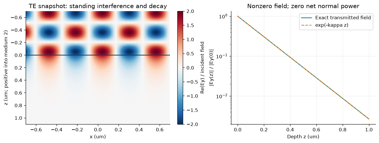
۳. دو بازتاب میتوانند خنثی شوند
لایه در تابش عمودی و دارد. مرجع میدان عبوری در صفحهٔ خروجی است، نه ورودی. برای و ، سهمهای بازتابی در طول موج طراحی خنثی میشوند. آیا توان عبوری واحد الزاماً میخواهد؟
wavelengths=np.linspace(.35,1.,391)
film_spectrum=film(N_INCIDENT,N_FILM,N_OUTPUT,THICKNESS_UM,wavelengths)
film_reference=film(N_INCIDENT,N_FILM,N_OUTPUT,THICKNESS_UM,WAVELENGTH_UM)
bare=interface(N_INCIDENT,N_OUTPUT,0.,'TE')
table(['Case','r','t at exit','|t|^2','R','T'],[['Bare interface',ctext(bare['r']),ctext(bare['t']),float(abs(bare['t'])**2),float(bare['R']),float(bare['T'])],['Quarter-wave film',ctext(film_reference['r']),ctext(film_reference['t']),float(abs(film_reference['t'])**2),float(film_reference['R']),float(film_reference['T'])]])
fig,axes=plt.subplots(1,2,figsize=(10.5,3.5),layout='constrained')
axes[0].plot(wavelengths,film_spectrum['R'],color=TEAL,label='Quarter-wave film')
axes[0].axhline(float(bare['R']),color=ORANGE,ls='--',label='Bare interface')
axes[0].set(xlabel='Vacuum wavelength (um)',ylabel='Reflected power fraction',title='Interference removes reflection at one wavelength');axes[0].legend()
axes[1].plot(wavelengths,np.rad2deg(np.unwrap(np.angle(film_spectrum['t']))),color=PURPLE)
axes[1].set(xlabel='Vacuum wavelength (um)',ylabel='Transmission phase at exit (deg)',title='Cancellation does not remove propagation phase')
for ax in axes:ax.axvline(WAVELENGTH_UM,color=NAVY,alpha=.4,lw=1);ax.grid(alpha=.2)
plt.show()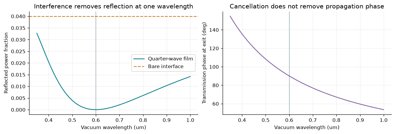
۴. نوک میدان الکتریکی را دنبال کنید
در نقطهٔ ثابت، بردار جونز واحد را بگیرید. با مسیر نوک میدان است. تعریف میکنیم و بهجای نام مبهم راستگرد یا چپگرد، قرارداد مختصات را گزارش میکنیم. تحلیلگر خطی در ، کسر را عبور میدهد.
tau=np.linspace(0.,2*np.pi,401);betas=np.linspace(0.,180.,361)
fig,axes=plt.subplots(1,2,figsize=(10,3.9),layout='constrained');jones_cases=[]
for delta,color in [(0.,TEAL),(45.,ORANGE),(90.,PURPLE)]:
    V=np.sin(2*np.deg2rad(JONES_ALPHA_DEG))*np.sin(np.deg2rad(delta))
    name='Linear' if abs(V)<1e-12 else ('Circular' if abs(abs(V)-1)<1e-12 else 'Elliptical')
    name+=f' (delta={delta:g} deg)'
    J=polarization(JONES_ALPHA_DEG,delta,0.)
    ex=np.real(J['Ex']*np.exp(-1j*tau));ey=np.real(J['Ey']*np.exp(-1j*tau))
    axes[0].plot(ex,ey,color=color,label=name)
    j=45;axes[0].annotate('',xy=(ex[j+12],ey[j+12]),xytext=(ex[j],ey[j]),arrowprops=dict(arrowstyle='->',color=color,lw=1.8))
    transmission=polarization(JONES_ALPHA_DEG,delta,betas)['analyzer_power']
    axes[1].plot(betas,transmission,color=color,label=name)
    jones_cases.append(dict(name=name,alpha_deg=JONES_ALPHA_DEG,delta_deg=delta,response=J))
axes[0].set(xlabel='Ex (normalized)',ylabel='Ey (normalized)',title='Field tip at a fixed point',xlim=(-.85,.85),ylim=(-.85,.85));axes[0].set_aspect('equal')
axes[1].set(xlabel='Linear analyzer angle (deg)',ylabel='Power / incident power',title='The analyzer converts polarization into intensity',ylim=(-.02,1.02))
for ax in axes:ax.grid(alpha=.2);ax.legend(fontsize=9)
plt.show()
table([f'State at alpha={JONES_ALPHA_DEG:g} deg','I','Q','U','V','Power through x analyzer'],[[c['name']]+[float(c['response'][k]) for k in ['I','Q','U','V','analyzer_power']] for c in jones_cases])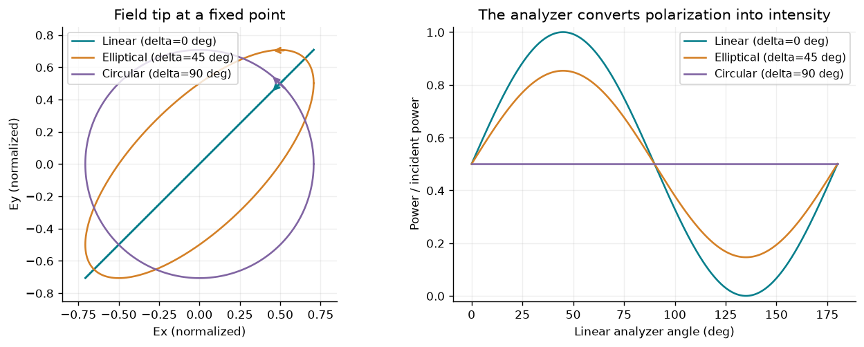
۵. فاز، جذب را کنترل میکند
برای ورقهٔ الکتریکی با صفحات منطبق در هوا، ، ، و . در ، یک موج فرودی و میدهد. دو ورودی همدوس همتوان با همان توان ورودی کل، پاسخ دارند. فاز میدان تعیین میکند کانال زوج اتلافی یا کانال فرد بیاتلاف تحریک شود.
این نتیجهٔ مدل مرزی ایدهآل است، نه جاذب ساختهشده. بازیابی جبری به معنادار و قید ورقهٔ نیاز دارد. آن را نمیتوان بیبررسی برای صفحات مرجع متفاوت لایهٔ متناهی استفاده کرد.
conductances=np.linspace(0.,8.,321);phases=np.linspace(0.,360.,361)
shunt_sweep=sheet(conductances,0.)
coherent_sweep=coherent_sheet(SHEET_G,SHEET_B,phases)
fig,axes=plt.subplots(1,2,figsize=(10.5,3.6),layout='constrained')
for key,color in [('R',ORANGE),('T',NAVY),('A',TEAL)]:axes[0].plot(conductances,shunt_sweep[key],color=color,label=key)
axes[0].axvline(2,color=PURPLE,ls='--',alpha=.5);axes[0].set(xlabel='Normalized conductance G (B=0)',ylabel='Fraction of incident power',title='One-sided electric sheet: A reaches 1/2');axes[0].legend()
axes[1].plot(phases,coherent_sweep['absorbed'],color=TEAL,label='Two coherent incident beams')
axes[1].axhline(float(sheet(SHEET_G,SHEET_B)['A']),color=ORANGE,ls='--',label='One-sided illumination')
axes[1].set(xlabel='Relative incident phase (deg)',ylabel='Absorbed fraction',title='Same total input power; different absorption');axes[1].legend(fontsize=9)
for ax in axes:ax.set_ylim(-.02,1.02);ax.grid(alpha=.2)
plt.show()
sheet_cases=[]
for G,B in [(0.,0.),(0.,2.),(.4,-1.),(2.,0.),(6.,0.)]:
    s=sheet(G,B);retrieved=retrieve_sheet(s['r'],s['t']);sheet_cases.append(dict(G=G,B=B,response=s,retrieved_g=retrieved))
table(['G','B','r','t','R','T','A','Retrieved g'],[[c['G'],c['B'],ctext(c['response']['r']),ctext(c['response']['t'])]+[float(c['response'][k]) for k in ['R','T','A']]+[ctext(c['retrieved_g'])] for c in sheet_cases])
table(['Relative phase (deg)','Two-beam absorbed fraction'],[[p,float(coherent_sheet(2.,0.,p)['absorbed'])] for p in [0.,90.,180.,270.]])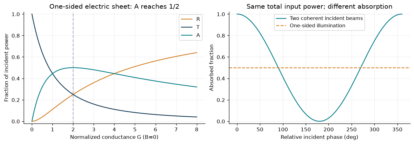
آزمایش کنترلشدهٔ خطای بازیابی
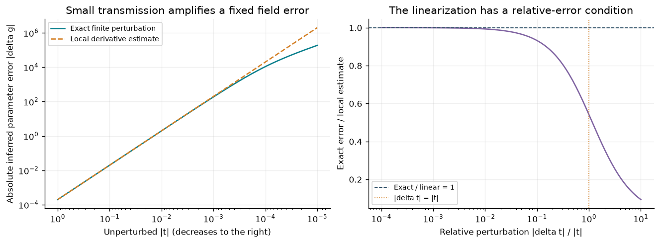
وارون حتی وقتی فرمول تحلیلی آن دقیق است حساسیت دارد. شنتهای حقیقی غیرفعال را در دو محیط هوای یکسان جاروب کنید و اغتشاش مختلطی با اندازهٔ مطلق ثابت به عبور بیفزایید. پیشبینی کنید با کوچک شدن عبور، خطای پارامتر استنباطشده چگونه تغییر میکند.
کد، تفاضل محدود دقیق را با برآورد موضعی مشتق مقایسه میکند. برآورد به کوچک بودن اغتشاش نسبت به عبور نیاز دارد؛ کوچک بودن آن نسبت به یک کافی نیست. بازتاب اغتشاشیافته را برابر عبور اغتشاشیافته منهای یک میگذاریم؛ پس این آزمایش حساسیت مصنوعی با مدل سازگار است. خطاهای مستقل اندازهگیری بازتاب و عبور میتوانند پیوستگی را نیز نقض کنند و باید جداگانه بررسی شوند؛ آنها را بیبررسی به این وارون تحمیل نمیکنیم.
اندازه و جهت اغتشاش را در کد تغییر دهید. نسبت اندازهٔ اغتشاش به عبور را گزارش کنید، محل شکست تقریب خطی را بیابید و پارامتر استنباطشده را از ورقهٔ غیرفعال اولیه متمایز کنید. همهٔ منحنیها محاسبات اصیل از وارون مشخصاند و دادهٔ اندازهگیری یا تمامموج ندارند.
# A deterministic synthetic perturbation, not a measurement-noise distribution.
RETRIEVAL_PERTURBATION = 1e-4
RETRIEVAL_DIRECTION_DEG = 45.
RETRIEVAL_MIN_TRANSMISSION = 1e-5
assert 0 < RETRIEVAL_PERTURBATION < .01
assert 0 < RETRIEVAL_MIN_TRANSMISSION < 1
assert np.isfinite(RETRIEVAL_DIRECTION_DEG)

nominal_amplitudes = np.geomspace(1., RETRIEVAL_MIN_TRANSMISSION, 161)
nominal_conductances = 2/nominal_amplitudes-2
nominal_sheet = sheet(nominal_conductances, 0.)
nominal_t = nominal_sheet['t'].astype(complex)
delta_t = RETRIEVAL_PERTURBATION*np.exp(1j*np.deg2rad(RETRIEVAL_DIRECTION_DEG))
perturbed_t = nominal_t+delta_t
perturbed_r = perturbed_t-1  # Deliberately preserve this synthetic model's continuity.
assert np.all(np.abs(perturbed_t) > 1e-8), 'Choose a perturbation away from the inverse singularity.'
retrieved_perturbed = retrieve_sheet(perturbed_r, perturbed_t)
parameter_error = np.abs(retrieved_perturbed-nominal_conductances)
finite_difference = 2*abs(delta_t)/(np.abs(nominal_t)*np.abs(perturbed_t))
linear_estimate = 2*abs(delta_t)/np.abs(nominal_t)**2
relative_perturbation = abs(delta_t)/np.abs(nominal_t)
assert np.allclose(parameter_error, finite_difference, rtol=1e-8, atol=1e-9)
small_perturbation = relative_perturbation <= .01
assert np.max(np.abs(parameter_error[small_perturbation]/linear_estimate[small_perturbation]-1)) < .011

fig, axes = plt.subplots(1, 2, figsize=(10.5, 3.8), layout='constrained')
axes[0].loglog(np.abs(nominal_t), parameter_error, color=TEAL, label='Exact finite perturbation')
axes[0].loglog(np.abs(nominal_t), linear_estimate, '--', color=ORANGE, label='Local derivative estimate')
axes[0].invert_xaxis()
axes[0].set(xlabel='Unperturbed |t| (decreases to the right)', ylabel='Absolute inferred parameter error |delta g|', title='Small transmission amplifies a fixed field error')
axes[1].semilogx(relative_perturbation, parameter_error/linear_estimate, color=PURPLE)
axes[1].axhline(1., color=NAVY, ls='--', lw=1, label='Exact / linear = 1')
axes[1].axvline(1., color=ORANGE, ls=':', lw=1, label='|delta t| = |t|')
axes[1].set(xlabel='Relative perturbation |delta t| / |t|', ylabel='Exact error / local estimate', title='The linearization has a relative-error condition')
for ax in axes:
    ax.grid(alpha=.2)
    ax.legend(fontsize=8)
plt.show()
selected_rows = np.linspace(0, len(nominal_t)-1, 6, dtype=int)
table(['Unperturbed |t|', '|delta t| / |t|', 'Exact |delta g|', 'Local estimate'],
      [[float(abs(nominal_t[j])), float(relative_perturbation[j]), float(parameter_error[j]), float(linear_estimate[j])] for j in selected_rows])
independent_continuity_residual = float(np.max(np.abs(perturbed_t-1-nominal_sheet['r'])))
print('Continuity residual if only transmission is perturbed:', independent_continuity_residual)
print('The plotted inverse instead uses model-consistent perturbed r=t-1; independent measurement noise needs its own residual/tolerance model.')
retrieval_conditioning = dict(perturbation_magnitude=RETRIEVAL_PERTURBATION,
    perturbation_direction_deg=RETRIEVAL_DIRECTION_DEG,
    nominal_t=nominal_t, nominal_g=nominal_conductances,
    perturbed_t=perturbed_t, perturbed_r=perturbed_r, retrieved_g=retrieved_perturbed,
    relative_perturbation=relative_perturbation, absolute_parameter_error=parameter_error,
    linear_estimate=linear_estimate, independent_continuity_residual=independent_continuity_residual,
    scope='Deterministic model-consistent sensitivity experiment; not measured noise or geometry retrieval')
Continuity residual if only transmission is perturbed: 0.00010000000000011169
The plotted inverse instead uses model-consistent perturbed r=t-1; independent measurement noise needs its own residual/tolerance model.
۶. کنترل و خروجیگیری
برای درگاههای منتشرشونده، دامنهٔ بهنجارشدهٔ توانی عامل دارد. ماتریس لایهٔ بیاتلاف باید یکانی و متقابل باشد؛ ورقهٔ اتلافی باید انقباضی باشد، یعنی توان خروجی برای هر ورودی از ورودی بیشتر نشود. اینها کنترل مدل تخت دقیقاند. حل مستقل چهار معادلهٔ مرزی لایه و بررسی گستردهتر پارامترها در scripts/validate_chapter02.py ارائه شده است.
normal=interface(1.,1.5,0.,'TE')
assert abs(normal['r']+.2)<1e-12 and abs(normal['t']-.8)<1e-12
assert abs(normal['T']-.96)<1e-12
S=film_scattering(N_INCIDENT,N_FILM,N_OUTPUT,THICKNESS_UM,wavelengths)
film_unitarity=float(np.max(abs(np.swapaxes(S.conj(),-1,-2)@S-np.eye(2))))
assert film_unitarity<1e-12
assert float(film_reference['R'])<1e-12
assert abs(float(sheet(2.,0.)['A'])-.5)<1e-12
assert abs(float(coherent_sheet(2.,0.,0.)['absorbed'])-1)<1e-12
assert abs(float(coherent_sheet(2.,0.,180.)['absorbed']))<1e-12
j=polarization(35.,61.,17.)
stokes_error=float(abs(j['I']**2-j['Q']**2-j['U']**2-j['V']**2));assert stokes_error<1e-12
def serial(value):
    if isinstance(value,dict):return {k:serial(v) for k,v in value.items()}
    if isinstance(value,(list,tuple)):return [serial(v) for v in value]
    if isinstance(value,np.ndarray):return serial(value.tolist())
    if isinstance(value,(complex,np.complexfloating)):return dict(re=serial(float(value.real)),im=serial(float(value.imag)))
    if isinstance(value,(float,np.floating)):return float(value) if np.isfinite(value) else None
    if isinstance(value,np.generic):return value.item()
    return value
metadata=dict(model_version=MODEL_VERSION,topic_ids=['ms-01-waves-interfaces','ms-03-sheet-response','ms-06-polarization'],source_sha256=hashlib.sha256((ROOT/'simulations/waves_interfaces.py').read_bytes()).hexdigest(),model='exact planar interface/film/electric-sheet and Jones models',time_convention='exp(-i omega t)',spatial_convention='exp(+i k.r)',amplitude_basis='common tangential electric field; reflected TM sign differs from a rotating local p basis',phase_planes=dict(interface='z=0',sheet='coincident sheet plane',film='entrance for r; exit for t'),bulk_model='positive real constant refractive indices, isotropic nonmagnetic media',limitations=['No patterned-geometry Maxwell solver','No measured dispersion or fabricated-device validation','Film and sheet at normal incidence','Jones analyzer is an ideal deterministic fully polarized model','Electric-sheet retrieval is algebra under explicit continuity and plane assumptions'],environment=dict(python=platform.python_version(),numpy=np.__version__,matplotlib=matplotlib.__version__))
data=dict(metadata=metadata,parameters=dict(n1=N_INCIDENT,n2=N_OUTPUT,nf=N_FILM,wavelength_um=WAVELENGTH_UM,thickness_um=THICKNESS_UM),interface_cases=interface_cases,angles_deg=ANGLES_DEG,angular=angular,field_checks=field_checks,film_benchmark=film_reference,wavelengths_um=wavelengths,film_spectrum=film_spectrum,jones_cases=jones_cases,sheet_cases=sheet_cases,conductances=conductances,sheet_sweep=shunt_sweep,relative_phases_deg=phases,coherent_sweep=coherent_sweep,retrieval_conditioning=retrieval_conditioning,checks=dict(film_unitarity_error=film_unitarity,stokes_error=stokes_error))
(DATA/'waves-reference.json').write_text(json.dumps(serial(data),indent=2,allow_nan=False)+'\n',encoding='utf-8')
with (DATA/'waves-reference.csv').open('w',newline='',encoding='utf-8') as handle:
    writer=csv.writer(handle);writer.writerow(['experiment','parameter','value','r_real','r_imag','t_real','t_imag','R','T','A','phase_deg'])
    def row(name,key,value,v,j):
        phase=float(v['phase_deg'][j]);writer.writerow([name,key,float(value),float(v['r'][j].real),float(v['r'][j].imag),float(v['t'][j].real),float(v['t'][j].imag),float(v['R'][j]),float(v['T'][j]),float(v.get('A',np.zeros_like(v['R']))[j]),'' if not np.isfinite(phase) else phase])
    for name,v in angular.items():
        for j,a in enumerate(ANGLES_DEG):row(name,'angle_deg',a,v,j)
    for j,w in enumerate(wavelengths):row('quarter_wave_film','wavelength_um',w,film_spectrum,j)
    for j,G in enumerate(conductances):row('electric_sheet_B0','conductance',G,shunt_sweep,j)
table(['Notebook check','Worst error'],[['Film power-normalized unitarity',film_unitarity],['Jones Stokes identity',stokes_error],['TIR normal flux',field_checks['max_transmitted_flux']]])
print('Saved strict JSON and CSV with source hash and explicit reference-plane/model conventions.')Saved strict JSON and CSV with source hash and explicit reference-plane/model conventions.
شگفتیها را توضیح دهید
دامنهٔ میدان را با توان عمودی، دامنهٔ مماسی صفر را با میدان اوانسنت ناصفر، و روشنسازی یکطرفه را با دوطرفه مقایسه کنید. چرا ضدبازتاب ربعموج گزارهای طیفی و وابسته به مرجع فاز است؟ چرا بازیابی ورقه پیش از محاسبهٔ جبری، آزمون اعتبار مدل است؟
استخراجهای فصل، مثالهای حلشده و آزمایشگاه را ببینید. فقط پس از تعیین هندسه، قطبش، کانالها، صفحات فاز و اعتبارسنجی عددی اضافی، این مبنا را به بررسی ریج فصل ۳ و پراش فصل ۴ تعمیم دهید؛ نسخهٔ فارسی هر دو فصل نیز در کتاب در دسترس است.