Chapter 6: Numerical Modeling and Simulation Methods

Can a calculation conserve power to fifteen digits and still predict the wrong transmitted wave? Yes. This chapter lets you produce that result, diagnose it, and improve it.

In Chapter 2, a planar film had an exact scattering solution. We now solve the same physical problem by finite differences and compare the results. The benchmark separates errors in the numerical method from uncertainty about the physical structure. We then revisit the harmonic refinements of Chapters 3 and 5.

Use the worked examples, interactive lab, and executed notebook. Prerequisites are Chapter 2, linear systems, and complex numbers; the RCWA comparison also uses Chapters 3–5. Study this methods strand before trusting a new response library.

A three-dimensional cut of the uniform film and a one-dimensional z grid, showing physical faces, incoming/reflected/transmitted waves and radiation boundaries. — The benchmark object is a uniform film, infinite along x and y: d = 0.60 µm, film index 2.4, exterior index 1.0. Numerical nodes are not extra layers. This reference sketch shows N = 8 and zero exterior padding; the explorer updates mesh and padding labels from its controls.

What you should learn¶

By the end, you should be able to choose a solver family for a specified geometry and observable, derive a small frequency-domain discretization, separate equation residual from prediction error, refine independent numerical controls, compare complex amplitudes at common reference planes, and write a reproducible acceptance statement.

Executed scope: a normal-incidence, one-dimensional, isotropic, nonmagnetic, lossless dielectric slab with equal exterior indices; a harmonic-refinement companion using the existing TE ridge solver. FEM, time-domain, finite-device, dispersive-material, and experimental comparisons below are further lab outlines.

Choose the problem before the solver¶

First specify illumination, material law, geometry, boundary conditions, the quantity to report, and an accuracy target. A large field image is useful only if its normalization, location, and numerical controls are known.

Method	Natural use in this course	Controls that need independent refinement
Exact planar/interface or sheet model	Limits, signs, phase planes, inexpensive design intuition	Physical approximation and parameter validity; no spatial mesh exists
RCWA / Fourier modal method	Periodic, layered structures and diffraction channels	Harmonic truncation, material Fourier representation; layer slicing when geometry varies along propagation
FDFD	A frequency-domain boundary-value problem on a spatial grid	Mesh, interface representation, boundaries, domain/monitor placement, linear solve
FEM	Vector fields on meshes fitted to complex geometries	Element size/order, curved geometry, ports/boundaries, solver tolerance
FDTD	Time-resolved fields and spectra from a time-domain excitation	Spatial/time steps, source spectrum, run duration, interface treatment, domain and absorbers
Surface integral / BEM	Scattering with suitable piecewise homogeneous regions	Surface mesh, quadrature, linear solve, and background Green function assumptions

The Meep introduction describes its space/time discretization. MFEM’s Maxwell notes explain tangentially conforming edge elements. SCUFF-EM’s implementation documentation describes surface-current discretization. These are method references; none of those packages is executed in this lab.

Our ridge RCWA code propagates modal fields analytically through a uniform layer. It has no time step or z mesh to refine. Comparing it with grcwa tests another implementation of the same method family. The new slab FDFD comparison exercises a different family, for the slab geometry only.

Four different questions about error¶

For a discrete system $A_h u_h=b_h$ and a reported complex transmission $t_h$ , define

\rho_h=\frac{\|A_hu_h-b_h\|_2}{\|b_h\|_2},\qquad \delta_P=|1-R_h-T_{h,\mathrm{net}}|,\qquad e_t=|t_h-t_{\mathrm{exact}}|.

(1)

The residual asks how closely we solved the assembled equations. Power balance checks a conservation identity of the discrete problem. The amplitude error asks how closely that problem predicts a known continuum solution. Model discrepancy asks whether either idealized problem describes a real device. Small values of the first two do not bound the last two.

Keep geometry, material uncertainty, discretization, artificial boundaries, algebraic solution, and observable extraction separate in an error budget. Their effects may be correlated; adding them in quadrature requires a justified statistical model. A missing polarization or a wrong material law survives mesh refinement.

Build a frequency-domain slab calculation¶

Use $e^{-i\omega t}$ , $k_0=2\pi/\lambda_0$ , and $E_y(z)$ at normal incidence. The slab occupies $0<z<d$ , with real indices $n_f$ inside and $n_e$ on both sides:

\frac{d^2 E}{dz^2}+k_0^2 n^2(z)E=0,\qquad E(z<0)=e^{ik_ez}+r e^{-ik_ez},\qquad E(z>d)=t e^{ik_e(z-d)},\qquad k_e=k_0n_e.

(2)

Thus $r$ is referenced to the entrance face and $t$ to the exit face. The incident field at the entrance has unit amplitude. The exact benchmark is Chapter 2’s independent Fresnel-film formula.

Place both faces on nodes, use $h=d/N$ , and replace the second derivative by a centered stencil:

E_{j-1}+\bigl[(k_0h)^2\varepsilon_j-2\bigr]E_j+E_{j+1}=0.

(3)

Interior nodes use $\varepsilon_j=n_f^2$ , exterior nodes use $n_e^2$ , and each face node uses $(n_f^2+n_e^2)/2$ . This interface average applies to our scalar tangential electric field and aligned slab; it is not a universal prescription for normal electric components, metals, curved corners, or general vector Maxwell equations.

A uniform exterior supports a discrete traveling wave with phase step $\theta$ :

4\sin^2(\theta/2)=(k_eh)^2,\qquad \theta=2\arcsin(k_eh/2),\qquad k_eh<2.

(4)

The grid cutoff is a mathematical domain limit, not an accuracy recommendation. Even safely below cutoff, numerical dispersion can be substantial. The implementation requires $k_0h\max(n_f,n_e)<2$ in both media. Admissible coarse grids may still be inaccurate and are retained to expose that failure.

The right outgoing ghost value is $E_{J+1}=e^{i\theta}E_J$ . On the left, add a known incident wave and impose outgoing behavior on the reflected part. These discrete outgoing boundaries are exact for the homogeneous exterior stencil. They are not a PML. A deliberately mismatched option uses $e^{ik_eh}$ on the right to reveal small artificial reflections.

See conservation fail as an accuracy certificate¶

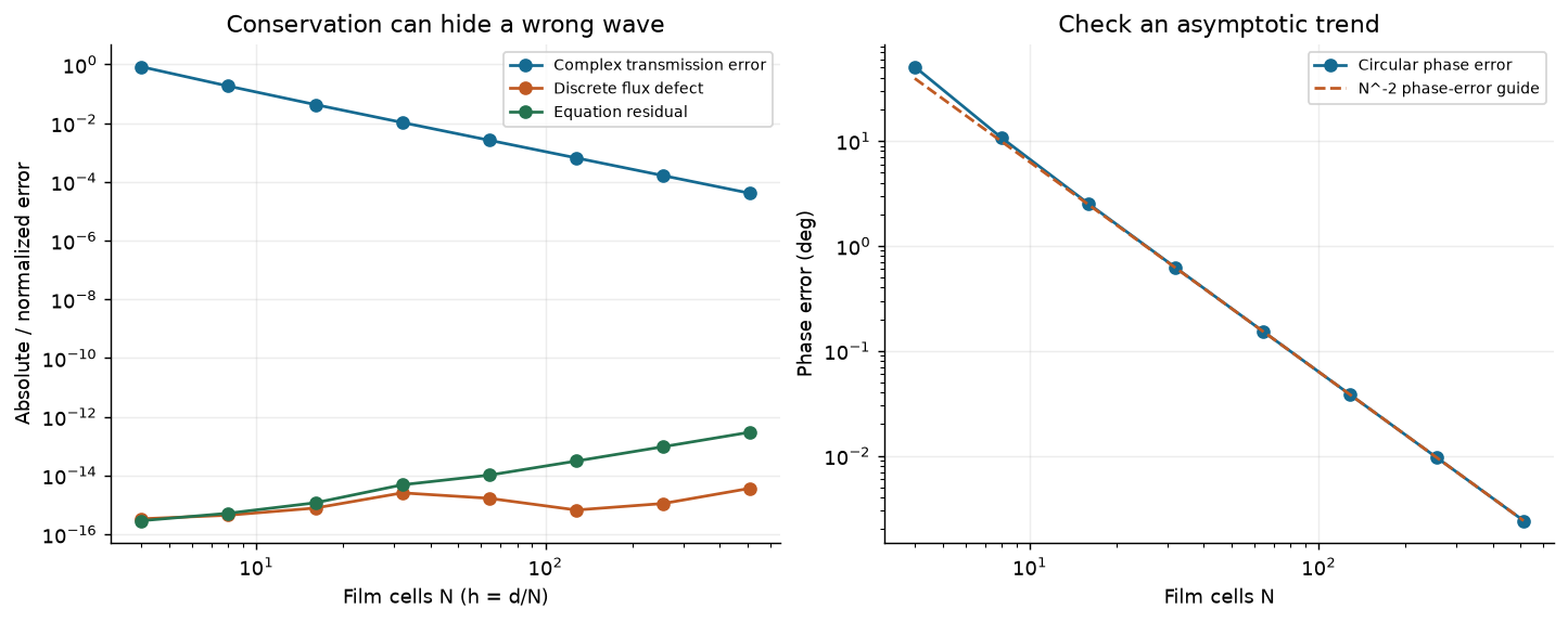
Logarithmic mesh-refinement plot comparing complex transmission error, algebraic residual, and discrete power imbalance. — Three diagnostics answer different questions. A coarse conservative system can have a tiny residual and power defect while its complex transmission remains inaccurate. The benchmark error falls with spatial refinement.

For the published slab, $\lambda_0=1.55\,\mu\mathrm m$ , $d=0.60\,\mu\mathrm m$ , $n_f=2.4$ , and $n_e=1$ . Predict which plotted curve will change most before doubling $N$ . Inspect circular phase error as well as power. Phase differences use $\arg(t_h t_{\rm exact}^*)$ , and cease to be informative near a transmission zero.

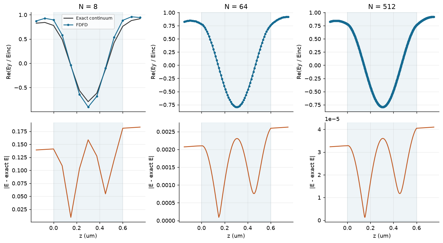
Real electric fields and pointwise errors for coarse and refined meshes compared with the exact slab field. — Field agreement is checked at the same physical coordinates and incident normalization. Fine grids improve phase accumulation and interference; the shaded interval is the physical film.

Move a monitor without moving the device¶

Suppose incident/reflected amplitudes are extracted at a left node a distance $L_-$ from the entrance and transmission at a right node $L_+$ after the exit. With local incident normalization, the raw coefficients satisfy

r_{\rm mon}=r_0 e^{2ik_hL_-},\qquad t_{\rm mon}=t_d e^{ik_h(L_-+L_+)},\qquad k_h=\theta/h.

(5)

Deembed using the same propagation law as the solved grid. Using continuum $k_e$ instead leaves an error proportional to $(k_h-k_e)L$ . Powers can remain unchanged while phase drifts. With the deliberately mismatched right boundary, forward and backward waves coexist in the output region; report their net flux separately. Here $t_{\rm mon}$ denotes the forward-wave coefficient obtained by decomposing the two traveling waves; the squared total field at one monitor node is not forward transmitted power.

J_{j+1/2}=\operatorname{Im}(E_j^*E_{j+1}),\qquad T_{\rm net}=T_{\rm forward}-T_{\rm backward}.

(6)

The grid current is constant in a real-index source-free region. It is proportional to physical flux in the continuum limit; normalization by the incident discrete current makes it the appropriate finite-grid conservation check. Equal exterior indices give the same current weight for incoming and outgoing amplitudes.

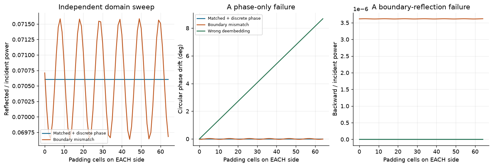
Independent padding sweep showing stable face-referenced amplitudes with matched boundaries, boundary-induced reflection, and phase drift from wrong deembedding. — Hold the film mesh fixed while varying padding. Correct discrete boundaries and deembedding give invariant face coefficients. Boundary mismatch and a reference-plane error leave distinct signatures.

In a larger FEM/FDTD simulation, open boundaries commonly use absorbing layers. PML performance still requires thickness and separation checks; see the Meep PML documentation. Do not move geometry, change mesh, and enlarge the absorber in one sweep and call the result a mesh-convergence study.

Estimate convergence and choose an acceptance target¶

If $Q_h=Q_*+Ch^p+o(h^p)$ over an asymptotic range, three equally refined meshes allow

p_{\rm obs}=\log_2\left|\frac{Q_h-Q_{h/2}}{Q_{h/2}-Q_{h/4}}\right|,\qquad Q_*\approx Q_{h/2}+\frac{Q_{h/2}-Q_h}{2^p-1}.

(7)

Apply this to a consistently defined observable, such as complex transmission, with care near cancellations and roundoff. These estimates require an observed asymptotic trend; they are not rigorous bounds. Discontinuities, geometry staircasing, corners, and changing material representations can alter the rate. Meep’s subpixel discussion gives examples of interface effects; our aligned scalar slab does not establish a universal second-order rate.

Select tolerances for the design decision before choosing a mesh. For example, a phase-sensitive library might require both $|\Delta t|<10^{-3}$ and a phase change below $0.1^\circ$ where transmission is appreciable. Test the worst relevant geometries and frequencies, rather than transferring one accepted mesh to every resonant structure.

Transfer the habit to patterned metasurfaces¶

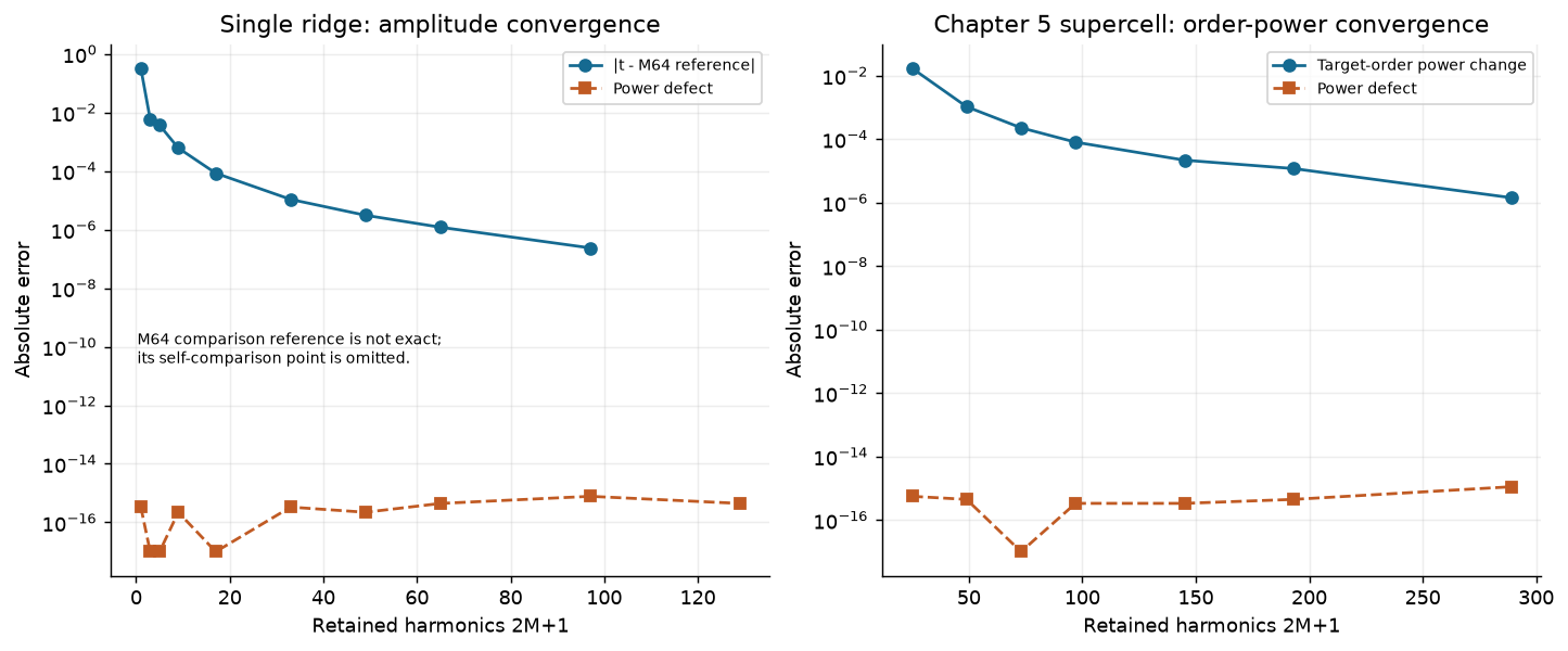
RCWA harmonic-refinement comparison of target-order power changes and numerical conservation diagnostics. — The Chapter 5 supercell also conserves power before its target-order power converges. The reference comparison uses higher-harmonic saved calculations; it is refinement evidence rather than an exact solution.

For a periodic ridge, refine harmonics while keeping geometry, material law, incidence, order definitions, and phase planes fixed. Check all propagating channels and the complex amplitude used for design. The highest retained calculation is a comparison reference, not mathematical truth. A second implementation tests software choices; a different method on the same geometry adds complementary evidence. A slab benchmark alone cannot validate a patterned supercell.

A reproducible simulation record¶

Record the physical problem, model omissions, units and phasor convention, solver/version/source hash, material data, numerical controls, source/monitor definitions, all power channels, independent refinements, acceptance criteria, and results including failed candidates. Archive the notebook and data used for each exported figure.

Before accepting your next design: explain which error was varied, what stayed fixed, why the comparison is independent, and which conclusions remain unsupported. Continue to Chapter 7’s tunable models when available; use these checks immediately in Chapters 3, 5, and 10.

Linked computational investigations¶

Continue with ms-09: spectral bandwidth, ms-10: independent cells versus supercells, and ms-11: bounded optimization with independent checks. These executed studies use the same explicit ridge geometry and connect spectral response, model approximation and design validation. The inverse-design study is a direct full-wave baseline for later AI comparisons.