Question: what can you predict before opening an electromagnetic solver?
Read Chapter 1, make predictions in the browser lab, and then inspect or run the notebook. The notebook and browser calculate an ideal sheet response; neither assigns a physical geometry.
Learning path
| Stage | Activity | Evidence to retain |
|---|---|---|
| 1 | Draw the structure and illumination | Element, pitch, period, aperture, and reference planes |
| 2 | Interpret complex coefficients | Amplitude, phase, and appropriate power normalization |
| 3 | Predict four sheet limits | A written prediction before using each preset |
| 4 | Change detuning and strength | Complex response and conservation checks |
| 5 | Examine frequency dependence | Phase plus amplitude, and a stated spectral metric |
| 6 | Compare evidence levels | An analytical claim, a full-wave claim, and their limits |
For a handmade demonstration, draw two complex arrows on movable cards. Arrange them head-to-tail to make zero, then align them to make a nonzero sum. Relate the construction to the model’s reflected and transmitted channel combinations. The cards illustrate complex addition; they do not measure the radiated fields of a physical meta-atom.
Example 1: wavelength in the relevant medium
At ,
In a real-index medium with , the wavelength is approximately . A dimension of is therefore about but in that medium. Always name the wavelength used in a “subwavelength” statement.
This conversion does not provide a homogenization theorem. Period, illumination, resonance, coupling, and the observable still determine whether an effective description is useful.
Example 2: the same power can have a different phase
For equal exterior impedances at normal incidence, and both give . Their phases differ by at the same reference plane. Interfering either field with a fixed reference can distinguish them.
The coefficient gives and phase in the same normalization. At , transmitted power is zero and phase is undefined. Reporting a phase there cannot establish a useful transmitted-wave design.
Prediction: if a solver reports only transmitted intensity, can it distinguish the first two coefficients? The intensity alone does not retain that relative phase.
Example 3: an electric-like resonance
At and nonzero electric-like strength, . With the magnetic-like channel disabled, , so
The ideal sheet reflects all incident power. Its reflected field has a sign change, while its transmitted phase is undefined. The notebook stores the missing phase as null/blank rather than treating it as a physical zero-degree phase.
Example 4: a balanced pair at resonance
Now match the two channels, so :
The two reflected contributions cancel, and the transmitted coefficient retains a phase relative to the transparent reference. The model can therefore illustrate unit transmission with nonzero phase. It does not identify a ridge width, material, or fabricated sample that achieves the response.
Change the magnetic-like resonance to while keeping illumination at . Predict whether cancellation remains, then inspect the detuned preset. The model remains lossless, so the response redistributes power between its two ports.
Example 5: two-sided illumination is a stronger check
For , take the normalized even input . Its output is multiplied by . The odd input is multiplied by .
Both eigenvalues have unit magnitude. Thus this model preserves power for arbitrary combinations of the two incoming waves, not only the one-sided reference. The audit verifies the full unitary matrix and a general complex two-sided excitation.
The equality for one incident direction would be insufficient by itself to establish every matrix constraint for a general proposed model.
Example 6: phase slope and delay
For the balanced model at resonance, the exact channel derivative gives
At and , the group delay is about . Reducing makes the spectral phase transition sharper and increases its peak delay. The notebook compares a numerical derivative with the closed form and keeps amplitude beside phase.
The derivative concerns this imposed balanced analytical channel. It does not establish material dispersion, an achromatic geometry, or a geometry-specific bandwidth.
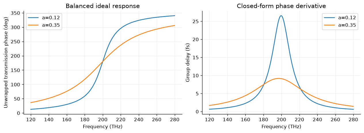
The executed notebook’s two balanced cases retain unit transmitted power by construction. Their different phase widths and delays concern this model, rather than a measured or simulated geometry bandwidth.
A bridge to saved full-wave data
For a worked comparison, inspect the first accepted row in the existing Chapter 3 TE ridge library. Its exterior indices are and , with real nonmagnetic media, normal incidence, and only the specular order open. For the electric-field transmission coefficient,
This follows from a normally incident propagating wave’s average flux and . The 0.08 μm ridge has but . Its reflected power is about 0.04006. Adding would incorrectly report missing power. These values can be checked directly from the saved complex coefficient in that Chapter 3 dataset: .
The ridge has height 0.60 μm, pitch 0.65 μm, wavelength 1.55 μm, and ridge/gap indices 2.4/1. Its transmission reference is at the layer exit, whereas the introductory sheet uses its single sheet plane. This worked arithmetic uses a previously executed full-wave result; it does not rerun Maxwell’s equations or retrieve a geometry-to-sheet mapping. Oblique incidence and more general media need the appropriate admittance factors developed in Chapter 2.
Reading a research result
Choose a metasurface figure or abstract and record the illumination, structure/material model, target quantity, normalization, and evidence level. Distinguish analytical, simulated, and experimental results. Check whether “efficiency” refers to incident power, transmitted power, one polarization, or a finite collection region.
For physical context, read Decker et al. on dielectric Huygens surfaces or Arbabi et al. on phase and polarization control. Their structures and measured/simulated results are external references, not outputs of this introductory model.
Report checklist
Submit predictions, parameter changes, complex coefficients, power and phase plots, assumptions, checks, and a paragraph describing a claim the model cannot support. A successful report can conclude that more geometry/material information is needed. The lab provides the runnable source and a bridge to existing full-wave results.
Use the self-check and mini-project page for answer guidance, a suggested grading rubric, a glossary, and an editable report worksheet.