Question: which parts of a wavefront design follow from a target formula, and which require a physical scattering calculation?
Use Chapter 5, the browser lab, and the two executed notebooks: beam steering and wavefront models. Their execution order matters: the wavefront notebook reads the expanded library produced by the beam notebook.
Learning path
| Stage | Prediction | Evidence |
|---|---|---|
| 1 | Sign and angle of the desired diffraction order | Phase gradient and Chapter 4 light cones |
| 2 | Whether a unit-cell library covers the target phases | Circular error and transmission threshold |
| 3 | Scattering of the selected geometry sequence | Local estimate versus full-wave order powers |
| 4 | Effect of identical cells and sequence reversal | Symmetry and mirror checks |
| 5 | Width and intensity of a finite scalar focus | Aperture propagation and window/grid refinements |
| 6 | Geometric phase and polarization leakage | Defined Jones/circular basis and retardance |
For a classroom demonstration, write six target phases on a circle. First select only from Chapter 3’s partial phase arc, then from the extended library. Compare the resulting geometry sequences before showing either full-wave spectrum. Ask students to predict the identical-cell and reversed-sequence controls.
Example 1: a six-cell beam direction
For and six cells, . At normal incidence, a positive ramp targets . With and output index 1.5,
Air-side reflection has orders -2 through +2, while glass-side transmission has -3 through +3. Their amplitudes cannot be obtained from this angle calculation. The six-ridge RCWA result supplies those amplitudes.
Example 2: six phase levels and their sinc factor
The staircase with has , so . This is a scalar coefficient fraction. The finite interval integration supplies the sinc; a point-source sum would omit that interval shape.
Compare this number with the actual supercell’s desired-order power. They refer to different models, and equality is not an acceptance condition. The audit checks the analytical coefficient identity for 2, 3, 4, 6, 8, and 16 levels.
Example 3: expand a library without hiding transmission constraints
The coarse height screen, using the original width domain, gives phase spans of approximately 132°, 200°, 271°, 341°, and 412° at heights 0.6, 0.9, 1.2, 1.5, and . These exploratory curves use ; the accepted library is recalculated and checked at higher order.
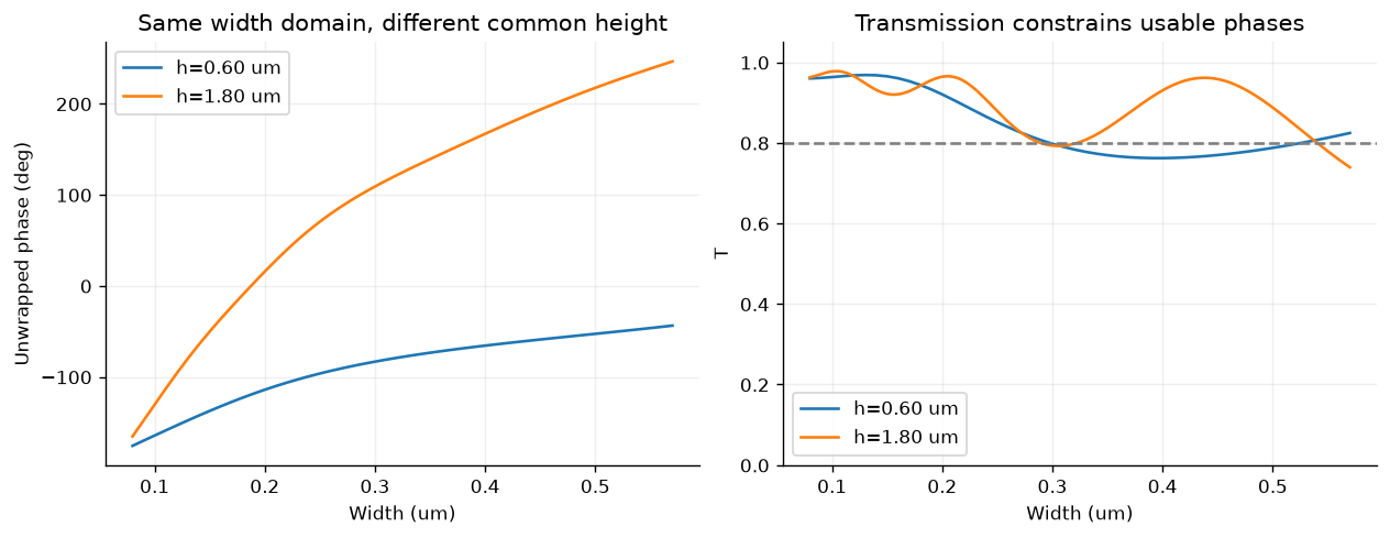
Increasing a common height expands phase coverage but also changes transmission. Use both quantities in selecting geometries.
A full unwrapped cycle does not guarantee every phase at . The six-target selection must still check each circular error. The saved expanded design has errors below at all six positions. It uses a common height, so the transmission reference plane is consistent within the sequence.
Example 4: two denominators for a beam’s performance
For the expanded supercell, and . Thus incident-normalized target power is approximately 85.54%, while
The second number excludes reflected incident power. Reporting it as incident efficiency would change the denominator. The local staircase predicts about 80.27% target power, and its reflected-plus-transmitted estimate is about 0.88225. That imbalance is an approximation error, not absorption in this lossless ridge model.
Example 5: identical elements and reversal
Six identical ridges preserve the smaller primitive period . In the expansion, only orders that are multiples of six can have nonzero amplitudes. At this wavelength none of the nonzero multiples is open, so all open nonzero supercell powers vanish.
For the selected asymmetric sequence, reversing widths mirrors the structure in . At normal incidence the transmitted/reflected order powers exchange . The strong +1 beam becomes a strong -1 beam. This is a symmetry check independent of whether the design objective was well chosen.
Example 6: a scalar line-focus metric
For , , and output index 1.5, the continuous focusing phase is . The saved scalar FWHM at the design plane is about for the continuous aperture, for the sampled phase aperture, and for the local-library aperture.
The local-library peak squared field is about 0.550 of the continuous reference peak. It includes amplitude reduction and phase/sampling effects. The fraction of modeled line intensity in a fixed window answers another question; it must not be relabeled as a full-wave lens efficiency. The window/grid checks concern propagation of these prescribed fields.
Example 7: a half-wave element at 30 degrees
With , , and element rotation , a state converts to with phase . The opposite input basis state gives phase .
If retardance is only , the ideal lossless retarder converts a fraction . Geometric-phase control and conversion amplitude require separate checks. These ideal Jones coefficients are not the vector response of our TE ridges.
Report checklist
Preserve target fields, phase/reference conventions, illumination, candidate library, selection objective, geometry sequence, local predictions, all-channel full-wave powers, numerical refinements, and control cases. For focusing/polarization, name the scalar or Jones model and its metrics. Retain lower-performing or infeasible cases when they reveal a limitation.
The lab specifies executed stages and further finite-device, independent-method, and optimization outlines. Chapter 6 broadens validation methods; Chapter 10 can reuse versioned simulation data for learned design.