Chapter 4 analytical notebook. Read the chapter, worked examples, and lab. The lab includes a browser explorer that runs directly on the published site.
This notebook computes allowed diffraction channels, analytical Fresnel power checks, and prescribed finite-array factors. It contains no patterned-device Maxwell solver and predicts no metasurface diffraction efficiency. All exterior indices are positive real numbers for homogeneous, isotropic, lossless media. Default lengths are in micrometers; angles are in degrees.
Restart the kernel and run all cells. Parameters are collected below. No external data, GPU, or network connection is needed during execution. For notebook sliders, install the book’s requirements-labs.txt and set ENABLE_WIDGETS=True; the reference saved outputs use False.
1. Parameters and environment
import sys
import json
import numpy as np
import matplotlib
import matplotlib.pyplot as plt
from matplotlib.colors import BoundaryNorm, ListedColormap
from IPython.display import display, HTML
from html import escape

PERIOD_UM, WAVELENGTH_UM = 3.0, 1.55
THETA_DEG, N_IN, N_OUT = 0.0, 1.0, 1.0
CUTOFF_TOL = 1e-10  # tolerance on abs(kx / (n_out*k0)) - 1
NEIGHBOR_ORDERS = 2
MAX_ENUMERATED_ORDERS = 10000
SWEEP_THETA = np.linspace(-70, 70, 281)
SWEEP_WAVELENGTH_UM = np.linspace(0.6, 3.6, 241)
ARRAY_SIZES = (8, 24, 64)
ARRAY_ANGLES_DEG = np.linspace(-89.9, 89.9, 9001)
ENABLE_WIDGETS = False

assert 0 < CUTOFF_TOL < 1e-3
assert isinstance(NEIGHBOR_ORDERS, int) and NEIGHBOR_ORDERS >= 1
assert all(isinstance(n, int) and n > 0 for n in ARRAY_SIZES)
assert np.isfinite(SWEEP_THETA).all() and np.all(np.abs(SWEEP_THETA) < 90)
assert np.isfinite(SWEEP_WAVELENGTH_UM).all() and np.all(SWEEP_WAVELENGTH_UM > 0)
print(f"Python {sys.version.split()[0]}; NumPy {np.__version__}; Matplotlib {matplotlib.__version__}")
print("Convention: exp(-i omega t), exp(i k.r), incidence from z<0; lengths in micrometers.")
print("Evidence: analytical channels, Fresnel interfaces, and prescribed scalar array factors.")

def show_table(headers, rows):
    header = "".join(f'<th scope="col">{escape(str(x))}</th>' for x in headers)
    body = "".join("<tr>" + "".join(f"<td>{escape(str(x))}</td>" for x in row) + "</tr>" for row in rows)
    display(HTML('<div style="overflow-x:auto;max-width:100%"><table><thead><tr>'+
                 header+'</tr></thead><tbody>'+body+'</tbody></table></div>'))
Python 3.12.1; NumPy 2.4.6; Matplotlib 3.11.1
Convention: exp(-i omega t), exp(i k.r), incidence from z<0; lengths in micrometers.
Evidence: analytical channels, Fresnel interfaces, and prescribed scalar array factors.
2. Define the channel calculation
The dimensionless tangential coordinate is
Compare with one. The positive outgoing-distance root is , with a positive imaginary part for closed channels. Reflected waves use the opposite laboratory sign because their outward direction points toward negative .
The open-order bounds come from solving for the integer . We use a conservative enclosing interval plus closed neighbors. This avoids silently dropping orders when the period or index grows. The explicit enumeration guard raises an error for an unreasonable array size rather than exhausting memory.
Near cutoff, the state is a tolerance-based classification. Its reported is the limiting grazing angle, not a finite-normal-power beam. Evanescent orders receive no real angle.
def validate_inputs(period_um, wavelength_um, theta_deg, n_in, n_out):
    values = np.array([period_um, wavelength_um, theta_deg, n_in, n_out], dtype=float)
    if not np.isfinite(values).all():
        raise ValueError("All physical parameters must be finite")
    if min(period_um, wavelength_um, n_in, n_out) <= 0:
        raise ValueError("Use positive period, wavelength, and real indices")
    if abs(theta_deg) >= 90:
        raise ValueError("Use an incidence angle strictly between -90 and 90 degrees")

def classify_q(q, n_out, tol=CUTOFF_TOL):
    distance = np.abs(np.asarray(q, dtype=float)/n_out)-1
    return np.where(distance < -tol, "open", np.where(distance > tol, "closed", "grazing"))

def floquet_orders(period_um, wavelength_um, theta_deg, n_in, n_out,
                   neighbors=NEIGHBOR_ORDERS, tol=CUTOFF_TOL):
    validate_inputs(period_um, wavelength_um, theta_deg, n_in, n_out)
    if not isinstance(neighbors, int) or neighbors < 1 or not 0 < tol < 1e-3:
        raise ValueError("Use at least one closed neighbor and a small positive cutoff tolerance")
    q_incident = n_in*np.sin(np.deg2rad(theta_deg))
    step = wavelength_um/period_um
    lower, upper = (-n_out-q_incident)/step, (n_out-q_incident)/step
    # Slightly expand by the classification tolerance so all near-grazing cases are included.
    padding = tol*n_out/step
    first = int(np.floor(lower-padding))-neighbors
    last = int(np.ceil(upper+padding))+neighbors
    if last-first+1 > MAX_ENUMERATED_ORDERS:
        raise ValueError("Too many orders for this teaching notebook; revise the parameter range")
    m = np.arange(first, last+1, dtype=int)
    q = q_incident + m*step
    state = classify_q(q, n_out, tol)
    kz_out_over_k0 = np.sqrt((n_out*n_out-q*q).astype(complex))
    angle = np.full(q.shape, np.nan)
    is_open, is_grazing = state == "open", state == "grazing"
    angle[is_open] = np.rad2deg(np.arcsin(q[is_open]/n_out))
    angle[is_grazing] = np.sign(q[is_grazing])*90
    assert np.all(kz_out_over_k0.real >= 0) and np.all(kz_out_over_k0.imag >= 0)
    return dict(m=m, q=q, state=state, angle_deg=angle,
                kz_out_over_k0=kz_out_over_k0, q_incident=q_incident)

def open_ids(result):
    return result["m"][result["state"] == "open"].tolist()

def print_channels(result, label):
    print(label, "open orders:", open_ids(result))
    show_table(["m", "kx/k0", "State", "Angle (degrees)", "Outward kz/k0"],
               [(int(m), f"{q:.6f}", state, "undefined" if np.isnan(angle) else f"{angle:.4f}", f"{kz:.5g}")
                for m, q, state, angle, kz in zip(result["m"], result["q"], result["state"],
                                                result["angle_deg"], result["kz_out_over_k0"])])

transmitted = floquet_orders(PERIOD_UM, WAVELENGTH_UM, THETA_DEG, N_IN, N_OUT)
reflected = floquet_orders(PERIOD_UM, WAVELENGTH_UM, THETA_DEG, N_IN, N_IN)
print_channels(transmitted, "Transmission region")
print("Reflection region open orders:", open_ids(reflected))
print("All table angles are channel directions; no amplitude or efficiency has been assigned.")
Transmission region open orders: [-1, 0, 1]
Reflection region open orders: [-1, 0, 1]
All table angles are channel directions; no amplitude or efficiency has been assigned.
3. Check independent analytical cases
The checks below cover known order sets and angles, exact cutoff and both sides of it, the decaying outgoing branch, Bloch-phase equivalence, input validation, and agreement with a much wider brute-force integer window. The latter checks enumeration, not the correctness of the physical formula by itself.
The microwave case uses mm and mm, corresponding to the rounded classroom convention m/s at 10 GHz. Converting both lengths to micrometers leaves their ratio unchanged.
reference = floquet_orders(3, 1.55, 0, 1, 1)
glass = floquet_orders(3, 1.55, 0, 1, 1.5)
primitive = floquet_orders(0.5, 1.55, 0, 1, 1)
assert open_ids(reference) == [-1, 0, 1]
assert open_ids(glass) == [-2, -1, 0, 1, 2]
assert open_ids(primitive) == [0]
assert np.isclose(reference["angle_deg"][reference["m"] == 1][0], 31.10892251052852)
assert np.isnan(reference["angle_deg"][reference["state"] == "closed"]).all()

cutoff_normal = floquet_orders(1.55, 1.55, 0, 1, 1)
assert cutoff_normal["m"][cutoff_normal["state"] == "grazing"].tolist() == [-1, 1]
assert open_ids(cutoff_normal) == [0]
cutoff_deg = float(np.rad2deg(np.arcsin(1.55/0.8-1.5)))
states = []
for offset in (-0.01, 0, 0.01):
    result = floquet_orders(0.8, 1.55, cutoff_deg+offset, 1, 1.5)
    states.append(result["state"][result["m"] == -1][0])
assert states == ["closed", "grazing", "open"]

microwave = floquet_orders(25000, 30000, 20, 1, 1)
assert open_ids(microwave) == [-1, 0]
microwave_angle = float(microwave["angle_deg"][microwave["m"] == -1][0])
assert np.isclose(microwave_angle, -59.09051239302117)
phase_advance = 2*np.pi*(25000/30000)*np.sin(np.deg2rad(20))
multiplier = np.exp(1j*phase_advance)
for m in microwave["m"]:
    assert np.allclose(np.exp(1j*(phase_advance+2*np.pi*m)), multiplier)

closed_index = int(np.flatnonzero(reference["m"] == 2)[0])
alpha_per_um = (2*np.pi/1.55)*reference["kz_out_over_k0"][closed_index].imag
assert alpha_per_um > 0
assert abs(np.exp(-alpha_per_um*2)) < abs(np.exp(-alpha_per_um)) < 1
# Reflected kz=-i*alpha: at z=-s, exp(i*kz*z)=exp(-alpha*s), also decaying.
assert np.isclose(abs(np.exp(1j*(-1j*alpha_per_um)*(-1))), np.exp(-alpha_per_um))

wide_m = np.arange(-200, 201)
for period, wavelength, theta, ni, no in [(3, 1.55, 0, 1, 1), (20, .5, 57, 1.2, 2),
                                         (.8, 1.55, -45, 1, 1.5), (1, 2, 65, 2, 1)]:
    result = floquet_orders(period, wavelength, theta, ni, no)
    q = ni*np.sin(np.deg2rad(theta)) + wide_m*wavelength/period
    expected = wide_m[classify_q(q, no) == "open"].tolist()
    assert open_ids(result) == expected

for invalid in [(0, 1, 0, 1, 1), (1, 1, 90, 1, 1), (1, 1, 0, -1, 1), (1, np.nan, 0, 1, 1)]:
    try:
        floquet_orders(*invalid)
    except ValueError:
        pass
    else:
        raise AssertionError("Invalid physical input was accepted")

validation_report = dict(air_open=open_ids(reference), glass_open=open_ids(glass),
                         primitive_open=open_ids(primitive), microwave_open=open_ids(microwave),
                         first_air_angle_deg=float(reference["angle_deg"][reference["m"] == 1][0]),
                         microwave_negative_angle_deg=microwave_angle,
                         microwave_phase_deg=float(np.rad2deg(phase_advance)),
                         cutoff_glass_deg=cutoff_deg, cutoff_sequence=states,
                         closed_m2_amplitude_decay_length_um=float(1/alpha_per_um))
print("Analytical channel, phase, branch, enumeration, and invalid-input checks passed.")
print(json.dumps(validation_report, indent=2))
Analytical channel, phase, branch, enumeration, and invalid-input checks passed.
{
  "air_open": [
    -1,
    0,
    1
  ],
  "glass_open": [
    -2,
    -1,
    0,
    1,
    2
  ],
  "primitive_open": [
    0
  ],
  "microwave_open": [
    -1,
    0
  ],
  "first_air_angle_deg": 31.10892251052852,
  "microwave_negative_angle_deg": -59.09051239302117,
  "microwave_phase_deg": 102.60604299770061,
  "cutoff_glass_deg": 25.94447977237001,
  "cutoff_sequence": [
    "closed",
    "grazing",
    "open"
  ],
  "closed_m2_amplitude_decay_length_um": 0.9475631587813499
}
4. Map channels across incidence and wavelength
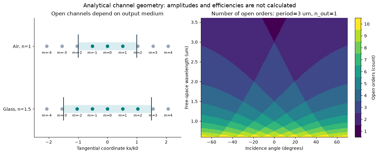
The left plot compares output light cones at one reference condition. The right plot counts open transmitted orders across the editable sweep. Grazing channels are not counted as ordinary open channels. The integer range is chosen from the entire sweep’s bounds, not only its initial wavelength or angle.
The constant indices here are teaching assumptions. For a dispersive material, evaluate its actual index at every wavelength. A channel-count color map is not an efficiency spectrum.
plt.rcParams.update({"font.size": 10, "axes.spines.top": False, "axes.spines.right": False})
fig, axes = plt.subplots(1, 2, figsize=(12, 4.8), constrained_layout=True)
ax = axes[0]
for row, (name, no) in enumerate([("Air output", 1.0), ("Glass output", 1.5)]):
    case = floquet_orders(PERIOD_UM, WAVELENGTH_UM, THETA_DEG, N_IN, no)
    ax.plot([-no, no], [row, row], color="#d9edf0", lw=18, solid_capstyle="butt")
    for m, q, state in zip(case["m"], case["q"], case["state"]):
        if abs(q) > 2.5:
            continue
        color = {"open": "#007d80", "grazing": "#b76a00", "closed": "#9ba7b5"}[state]
        ax.plot(q, row, "o", color=color, ms=7)
        ax.text(q, row+0.12, f"m={m}", ha="center", fontsize=8)
    ax.plot([-no, -no], [row-.18, row+.18], color="#182c42")
    ax.plot([no, no], [row-.18, row+.18], color="#182c42")
ax.set(xlabel="Tangential coordinate kx/k0", yticks=[0, 1], yticklabels=["Air, n=1", "Glass, n=1.5"],
       xlim=(-2.5, 2.5), ylim=(-.45, 1.45), title="Open channels depend on output medium")
ax.invert_yaxis()

q_inc = N_IN*np.sin(np.deg2rad(SWEEP_THETA))
step_min = np.min(SWEEP_WAVELENGTH_UM)/PERIOD_UM
max_order = int(np.ceil((N_OUT+np.max(np.abs(q_inc)))/step_min))+NEIGHBOR_ORDERS
if 2*max_order+1 > MAX_ENUMERATED_ORDERS:
    raise ValueError("Sweep requires too many diffraction orders")
count_map = np.zeros((len(SWEEP_WAVELENGTH_UM), len(SWEEP_THETA)), dtype=int)
for m in range(-max_order, max_order+1):
    q = q_inc[None, :] + m*SWEEP_WAVELENGTH_UM[:, None]/PERIOD_UM
    count_map += classify_q(q, N_OUT) == "open"
assert np.isfinite(count_map).all()
levels = np.arange(count_map.min()-.5, count_map.max()+1.5)
cmap = plt.get_cmap("viridis", len(levels)-1)
im = axes[1].pcolormesh(SWEEP_THETA, SWEEP_WAVELENGTH_UM, count_map, shading="auto",
                        cmap=cmap, norm=BoundaryNorm(levels, cmap.N))
axes[1].set(xlabel="Incidence angle (degrees)", ylabel="Free-space wavelength (um)",
            title=f"Number of open orders: period={PERIOD_UM:g} um, n_out={N_OUT:g}")
fig.colorbar(im, ax=axes[1], label="Open orders (count)", ticks=np.arange(count_map.min(), count_map.max()+1))
fig.suptitle("Analytical channel geometry: amplitudes and efficiencies are not calculated", fontsize=13)
plt.show()
5. Check power with a flat interface
For a nonmagnetic TE flat interface, let and on the outgoing branch. Then
The normalization factor is essential. In total internal reflection, is imaginary, so the outgoing evanescent field has zero normal transmitted power and . This analytical benchmark is independent of a future patterned-grating simulation. An artificial periodic box cannot make a flat interface excite non-specular orders.
def fresnel_te(n_in, n_out, theta_deg):
    validate_inputs(1, 1, theta_deg, n_in, n_out)
    zi = n_in*np.cos(np.deg2rad(theta_deg))
    q = n_in*np.sin(np.deg2rad(theta_deg))
    zt = np.sqrt(complex(n_out*n_out-q*q))
    r, t = (zi-zt)/(zi+zt), 2*zi/(zi+zt)
    return r, t, float(abs(r)**2), float(zt.real/zi*abs(t)**2)

normal = fresnel_te(1, 1.5, 0)
tir = fresnel_te(1.5, 1, 60)
assert np.allclose(normal, [-.2, .8, .04, .96])
assert np.isclose(tir[2], 1) and np.isclose(tir[3], 0)
max_power_residual = 0.0
for ni, no in [(1, 1.5), (1.5, 1), (1, 1)]:
    for theta in np.linspace(-80, 80, 161):
        _, _, R, T = fresnel_te(ni, no, theta)
        max_power_residual = max(max_power_residual, abs(R+T-1))
assert max_power_residual < 1e-12
show_table(["Interface case", "r (field)", "t (field)", "R (power)", "T (power)"],
           [(name, f"{r:.6g}", f"{t:.6g}", f"{R:.6g}", f"{T:.6g}")
            for name, (r, t, R, T) in [("Normal: 1 to 1.5", normal), ("TIR: 1.5 to 1, 60 deg", tir)]])
print(f"Maximum Fresnel power residual over 483 analytical checks: {max_power_residual:.3e}")
Maximum Fresnel power residual over 483 analytical checks: 4.441e-16
6. Finite arrays have finite angular widths
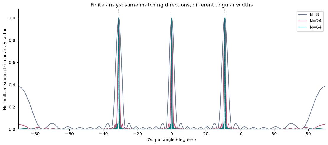
Use the directly evaluated scalar factor
All source weights are prescribed and equal after accounting for incident phase. There is no element pattern, coupling calculation, or electromagnetic boundary solution. The vertical markers below are open Floquet directions from the same physical parameters. A normalized squared scalar sum is not a power-normalized diffraction efficiency.
def array_factor(theta_deg, n_elements, period_um, wavelength_um, theta_incident, n_in, n_out):
    validate_inputs(period_um, wavelength_um, theta_incident, n_in, n_out)
    phase = (2*np.pi*period_um/wavelength_um)*(
        n_in*np.sin(np.deg2rad(theta_incident))-n_out*np.sin(np.deg2rad(np.asarray(theta_deg))))
    return np.mean(np.exp(1j*np.arange(n_elements)[:, None]*np.atleast_1d(phase)[None, :]), axis=0)

fig, ax = plt.subplots(figsize=(11, 4.8), constrained_layout=True)
for size, color in zip(ARRAY_SIZES, ("#64748b", "#b64d73", "#007d80")):
    factor = array_factor(ARRAY_ANGLES_DEG, size, PERIOD_UM, WAVELENGTH_UM, THETA_DEG, N_IN, N_OUT)
    assert np.max(np.abs(factor)) <= 1+1e-12
    ax.plot(ARRAY_ANGLES_DEG, np.abs(factor)**2, color=color, label=f"N={size}")
for angle in transmitted["angle_deg"][transmitted["state"] == "open"]:
    ax.axvline(angle, color="#182c42", ls=":", lw=1)
    for size in ARRAY_SIZES:
        at_order = array_factor([angle], size, PERIOD_UM, WAVELENGTH_UM, THETA_DEG, N_IN, N_OUT)
        assert np.allclose(np.abs(at_order), 1, atol=1e-12)
ax.set(xlabel="Output angle (degrees)", ylabel="Normalized squared scalar array factor",
       title="Finite arrays: same matching directions, different angular widths", xlim=(-90, 90), ylim=(0, 1.08))
ax.legend()
plt.show()
print("Array-factor values equal one at every open Floquet direction, within floating-point tolerance.")
Array-factor values equal one at every open Floquet direction, within floating-point tolerance.
7. Extend the channel test to a rectangular lattice
For periods and incident azimuth ,
Classify against , not alone. A circular light cone replaces the one-dimensional interval. This small example enumerates all potentially open pairs inside conservative bounds. It does not simulate a two-dimensional grating.
def rectangular_orders(px, py, wavelength, theta, phi, ni, no):
    validate_inputs(px, wavelength, theta, ni, no)
    validate_inputs(py, wavelength, theta, ni, no)
    if not np.isfinite(phi):
        raise ValueError("Azimuth must be finite")
    q = ni*np.sin(np.deg2rad(theta))
    qx0, qy0 = q*np.cos(np.deg2rad(phi)), q*np.sin(np.deg2rad(phi))
    lo_x, hi_x = int(np.floor((-no-qx0)*px/wavelength))-1, int(np.ceil((no-qx0)*px/wavelength))+1
    lo_y, hi_y = int(np.floor((-no-qy0)*py/wavelength))-1, int(np.ceil((no-qy0)*py/wavelength))+1
    if (hi_x-lo_x+1)*(hi_y-lo_y+1) > MAX_ENUMERATED_ORDERS:
        raise ValueError("Too many 2D orders for this teaching example")
    result = []
    for m in range(lo_x, hi_x+1):
        for n in range(lo_y, hi_y+1):
            qx, qy = qx0+m*wavelength/px, qy0+n*wavelength/py
            radius = np.hypot(qx, qy)
            state = str(classify_q(radius, no))
            result.append((m, n, qx, qy, state))
    return result

pairs = rectangular_orders(.8, 1.2, 1.55, 45, 0, 1, 1.5)
open_pairs = {(m, n) for m, n, _, _, state in pairs if state == "open"}
assert open_pairs == {(-1, 0), (0, -1), (0, 0), (0, 1)}
assert {(m, n) for m, n, _, _, s in rectangular_orders(.8, 1.2, 1.55, 45, 0, 1, 1) if s == "open"} == {(0, 0)}
print("Open rectangular-lattice orders in index 1.5:", sorted(open_pairs))
show_table(["m", "n", "kx/k0", "ky/k0", "State"],
           [(m, n, f"{qx:.6f}", f"{qy:.6f}", state) for m, n, qx, qy, state in pairs if state != "closed"])
Open rectangular-lattice orders in index 1.5: [(-1, 0), (0, -1), (0, 0), (0, 1)]
8. Optional Jupyter sliders
The saved reference output below is a short status message. Set ENABLE_WIDGETS=True in the first cell, restart, and run the notebook in Jupyter to enable controls. The sliders reuse the same floquet_orders function. The public lab’s standalone HTML explorer provides immediate browser interaction without a Python kernel.
if ENABLE_WIDGETS:
    import ipywidgets as widgets

    def explore(period_um, wavelength_um, theta_deg, n_in, n_out):
        result = floquet_orders(period_um, wavelength_um, theta_deg, n_in, n_out)
        print_channels(result, "Selected output region")

    controls = widgets.interactive(
        explore,
        period_um=widgets.FloatSlider(value=PERIOD_UM, min=.4, max=5, step=.01, description="Period (um)", continuous_update=False),
        wavelength_um=widgets.FloatSlider(value=WAVELENGTH_UM, min=.4, max=4, step=.01, description="Lambda (um)", continuous_update=False),
        theta_deg=widgets.FloatSlider(value=THETA_DEG, min=-75, max=75, step=.5, description="Angle (deg)", continuous_update=False),
        n_in=widgets.FloatSlider(value=N_IN, min=1, max=2.5, step=.05, description="n incident", continuous_update=False),
        n_out=widgets.FloatSlider(value=N_OUT, min=1, max=2.5, step=.05, description="n output", continuous_update=False))
    display(controls)
else:
    print("Reference execution complete. Set ENABLE_WIDGETS=True in Jupyter for sliders, or use the browser explorer in the lab.")
Reference execution complete. Set ENABLE_WIDGETS=True in Jupyter for sliders, or use the browser explorer in the lab.
9. Interpret the evidence
Report the open sets and signed angles for the optical and microwave cases; explain the cutoff tests, Fresnel normalization, and finite-array model limits. Include one proposed full-wave comparison using the lab’s interface or ridge-grating outline.
For extensions, vary the period or output index, implement a material-dispersion curve, or compare the scalar factors with a documented element pattern. Keep analytical, prescribed-model, full-wave, and measured results clearly identified. A successful channel calculation does not establish that a designed metasurface excites the desired channel efficiently.