دفترچهٔ فصل ۶: اعتماد به محاسبهٔ موج
ابتدا پیشبینی کنید: آیا دستگاهی پایسته میتواند موج اشتباهی را دقیق حل کند؟ لایهٔ دیالکتریک یکبعدی در تابش عمودی را با FDFD حل و با لایهٔ فرنل مستقل فصل ۲ مقایسه میکنیم. قرارداد است؛ میدان فرودی در ، دامنهٔ بازتاب در و عبور در تعریف میشوند. ضریبهای بیرونی حقیقی و برابر، ماده همسانگرد و غیرمغناطیسی و واحد طول میکرومتر است. اینجا PML، FDTD، FEM، آرایهٔ تیغهٔ محدود، پاشندگی ماده یا آزمایش تجربی اجرا نمیشود.
هسته را دوباره راهاندازی و همهٔ سلولها را اجرا کنید. بستهٔ منبع را کامل حفظ کنید. برچسب نمودارها در هر دو ویرایش انگلیسی علمی مشترکاند؛ متن فارسی معنای آنها را توضیح میدهد.
# Parameters: physical experiment and numerical controls are separate.
from dataclasses import asdict
from pathlib import Path
import hashlib, json, platform, sys
import numpy as np
import scipy
import matplotlib
import matplotlib.pyplot as plt
from IPython.display import HTML, display

ROOT = Path.cwd()
if not (ROOT / 'simulations').is_dir(): ROOT = ROOT.parent
assert (ROOT / 'simulations/numerical_methods.py').is_file(), 'Extract the complete source bundle.'
sys.path.insert(0, str(ROOT / 'simulations'))
from numerical_methods import Slab, solve_slab, exact_slab, exact_slab_fields, phase_error_deg, summarize_result

SLAB = Slab(wavelength_um=1.55, thickness_um=0.60, n_film=2.4, n_exterior=1.0)
MESH_CELLS = [4, 8, 16, 32, 64, 128, 256, 512]
FIELD_CELLS = [8, 64, 512]
PADDING_MESH = 8
PADDING_CELLS = list(range(65))
AMPLITUDE_TARGET = 1e-3
PHASE_TARGET_DEG = 0.1
PHASE_AMPLITUDE_FLOOR = 1e-8

plt.rcParams.update({'figure.dpi': 130, 'font.size': 10, 'axes.spines.top': False,
                     'axes.spines.right': False, 'axes.grid': True, 'grid.alpha': .22})
COLORS = ['#156a91', '#c05a23', '#25734f']
reference = exact_slab(SLAB)
print('Physical parameters:', asdict(SLAB))
print('Python / NumPy / SciPy / Matplotlib:', platform.python_version(), np.__version__, scipy.__version__, matplotlib.__version__)
print('Source SHA256:', hashlib.sha256((ROOT/'simulations/numerical_methods.py').read_bytes()).hexdigest())
print('Exact r, t, R, T:', reference['r'], reference['t'], reference['R'], reference['T'])
Physical parameters: {'wavelength_um': 1.55, 'thickness_um': 0.6, 'n_film': 2.4, 'n_exterior': 1.0}
Python / NumPy / SciPy / Matplotlib: 3.12.1 2.4.6 1.18.1 3.11.1
Source SHA256: 24f0cc7c187c6c92ba906aea101024b3249be87a2bae86c9ad148c79e7c0dd51
Exact r, t, R, T: (-0.2195960689010276-0.3261968489579452j) (0.7627137674043337-0.5134597270137267j) 0.15462681774687742 0.8453731822531227
۱. سه شاخص را جدا کنید
خطای عبور مختلط، باقیماندهٔ نرمالشدهٔ معادله و نقص شار گسسته را مستقل حساب کنید. جواب دقیق برای سنجش پیشبینی عددی است و در مونتاژ معادلات FDFD استفاده نمیشود. پیشبینی کنید آیا نقص توان با همان نرخ خطای عبور کاهش مییابد.
برای نمایش لگاریتمی، شاخصهای صفر یا کمتر از 1e-17 در کف ترسیم 1e-17 نشان داده میشوند؛ این کف مقدار خطای اندازهگیریشده نیست.
solutions = [solve_slab(SLAB, cells=n) for n in MESH_CELLS]
mesh = [summarize_result(s, reference) for s in solutions]
rows = ''.join(f"<tr><td>{r['cells']}</td><td>{r['complex_t_error']:.4g}</td><td>{r['phase_error_deg']:.5g}</td><td>{r['energy_defect']:.2e}</td><td>{r['algebraic_residual']:.2e}</td></tr>" for r in mesh)
display(HTML('<table><tr><th>Film cells N</th><th>|t - exact|</th><th>Phase error (deg)</th><th>Flux defect</th><th>Equation residual</th></tr>'+rows+'</table>'))
accepted = [r for r in mesh if r['complex_t_error'] < AMPLITUDE_TARGET and abs(r['phase_error_deg']) < PHASE_TARGET_DEG and abs(reference['t']) > PHASE_AMPLITUDE_FLOOR]
print('First sampled mesh meeting BOTH targets:', accepted[0]['cells'] if accepted else 'None: refine further')
for a,b in zip(mesh[-4:-1], mesh[-3:]):
    print(f"N {a['cells']} -> {b['cells']}: exact-error observed order {np.log2(a['complex_t_error']/b['complex_t_error']):.5f}")
assert max(r['algebraic_residual'] for r in mesh) < 1e-9
assert max(r['energy_defect'] for r in mesh) < 1e-9First sampled mesh meeting BOTH targets: 128
N 64 -> 128: exact-error observed order 2.00159
N 128 -> 256: exact-error observed order 2.00040
N 256 -> 512: exact-error observed order 2.00010
fig, ax = plt.subplots(1, 2, figsize=(11, 4.3), layout='constrained')
N = np.array(MESH_CELLS)
for key,label,color in [('complex_t_error','Complex transmission error',COLORS[0]), ('energy_defect','Discrete flux defect',COLORS[1]), ('algebraic_residual','Equation residual',COLORS[2])]:
    ax[0].loglog(N, np.maximum([r[key] for r in mesh], 1e-17), 'o-', color=color, label=label)
ax[0].set(xlabel='Film cells N (h = d/N)', ylabel='Absolute / normalized error', title='Conservation can hide a wrong wave')
ax[0].legend(fontsize=8)
ax[1].loglog(N, np.abs([r['phase_error_deg'] for r in mesh]), 'o-', color=COLORS[0], label='Circular phase error')
ax[1].loglog(N, abs(mesh[-1]['phase_error_deg'])*(N[-1]/N)**2, '--', color=COLORS[1], label='N^-2 phase-error guide')
ax[1].set(xlabel='Film cells N', ylabel='Phase error (deg)', title='Check an asymptotic trend')
ax[1].legend(fontsize=8)
plt.show()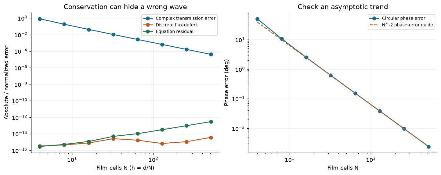
۲. میدان را در مختصات یکسان مقایسه کنید
دو وجه فیزیکی روی گرهها میمانند. هر وجه فقط برای این میدان اسکالر مماسی از میانگین حسابی گذردهی نیمسلول استفاده میکند. فاصلهٔ بیرونی هر طرف یکچهارم ضخامت لایه است. میدان حقیقی و خطای مختلط نقطهای را رسم کنید؛ شباهت شدت آزمونی ضعیفتر از توافق میدان مختلط است.
fig, axes = plt.subplots(2, len(FIELD_CELLS), squeeze=False, figsize=(11, 6), sharex='col', layout='constrained')
for col,n in enumerate(FIELD_CELLS):
    s = solve_slab(SLAB, cells=n, left_padding_cells=n//4, right_padding_cells=n//4)
    z, E = s['z_um'], s['E']
    exact_E = exact_slab_fields(SLAB, z)
    axes[0,col].plot(z, exact_E.real, color='0.2', label='Exact continuum')
    axes[0,col].plot(z, E.real, '.-', color=COLORS[0], label='FDFD')
    axes[0,col].set(title=f'N = {n}', ylabel='Re(Ey / Einc)')
    axes[1,col].plot(z, abs(E-exact_E), color=COLORS[1])
    axes[1,col].set(xlabel='z (um)', ylabel='|E - exact E|')
    for a in axes[:,col]: a.axvspan(0, SLAB.thickness_um, color=COLORS[0], alpha=.07)
axes[0,0].legend(fontsize=8)
plt.show()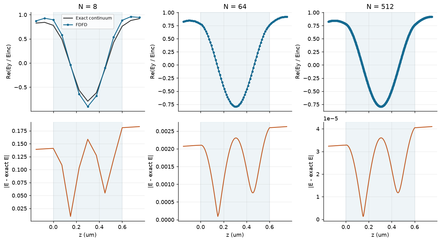
۳. مرز را حرکت دهید؛ شبکهٔ لایه ثابت بماند
سه تغییر جدا را بیازمایید: مرز تطبیقیافته با حذف فاز درست؛ ضریب خروجی راست عمداً اشتباه؛ مرز درست همراه حذف فاز پیوسته. توان رفت منهای برگشت، شار عبوری خالص است. مرز نامنطبق نمایش خطای کنترلشده است، نه جاذب جایگزین معتبر.
baseline = solve_slab(SLAB, cells=PADDING_MESH)
padding = []
cases = [('discrete','discrete','Matched + discrete phase'), ('continuum','discrete','Boundary mismatch'), ('discrete','continuum','Wrong deembedding')]
for boundary,deembed,label in cases:
    for p in PADDING_CELLS:
        s = solve_slab(SLAB, cells=PADDING_MESH, left_padding_cells=p, right_padding_cells=p, right_boundary=boundary, deembed=deembed)
        row = summarize_result(s, reference)
        row.update(label=label, padding_cells=p, complex_t_change=abs(s['t']-baseline['t']), phase_drift_deg=float(phase_error_deg(s['t'],baseline['t'])))
        padding.append(row)
fig, axes = plt.subplots(1,3,figsize=(12,4),layout='constrained')
for (_,_,label),color in zip(cases,COLORS):
    selected=[r for r in padding if r['label']==label]
    for a,key in zip(axes,['R','phase_drift_deg','T_backward']):
        if a is axes[0] and label == 'Wrong deembedding': continue
        a.plot(PADDING_CELLS,[r[key] for r in selected],color=color,label=label)
axes[0].set(ylabel='Reflected / incident power',title='Independent domain sweep')
axes[1].set(ylabel='Circular phase drift (deg)',title='A phase-only failure')
axes[2].set(ylabel='Backward / incident power',title='A boundary-reflection failure')
for a in axes:a.set_xlabel('Padding cells on EACH side')
axes[0].legend(fontsize=7)
axes[1].legend(fontsize=7)
plt.show()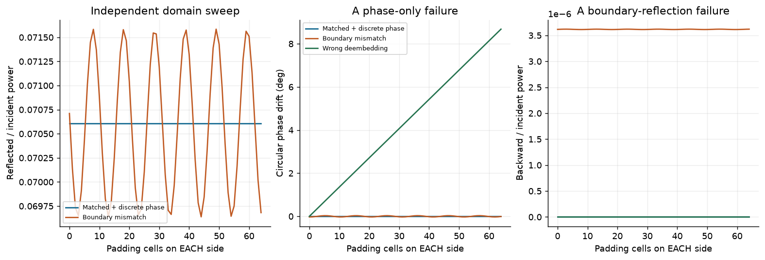
۴. مقایسهٔ خانوادهٔ گسستهسازی دیگر
نمودارهای بعد مجموعهدادهٔ RCWA منتشرشده با هندسهٔ ثابت را بررسی میکنند و پارامترهای قابل ویرایش لایهٔ بالا را به ارث نمیبرند. چپ: پیمایش تازهٔ هارمونیک تیغهٔ تکی از ممیزی فصل ۶ در مقایسه با نیممرتبهٔ M=64. راست: ابرسلول انحراف پرتو توسعهیافتهٔ ذخیرهشدهٔ فصل ۵ در مقایسه با کنترل مرتبهبالاتر آن. هیچ مرجع مرتبهبالاتری جواب دقیق نیست. هر دو مثال پایستگی پیش از همگرایی دامنه یا توان مرتبه را نشان میدهند.
fixed = json.loads((ROOT/'data/chapter-06/numerical-reference.json').read_text(encoding='utf-8'))
for name,digest in fixed['metadata']['source_sha256'].items():
    assert hashlib.sha256((ROOT/'simulations'/name).read_bytes()).hexdigest()==digest, 'Rerun the Chapter 6 audit after solver changes.'
harmonics = fixed['harmonics']
supercell = json.loads((ROOT/'data/chapter-05/beam-steering.json').read_text(encoding='utf-8'))
refinements = supercell['convergence']
fig, axes = plt.subplots(1,2,figsize=(11,4.5),layout='constrained')
axes[0].semilogy([r['retained_harmonics'] for r in harmonics[:-1]],np.maximum([r['complex_t_error'] for r in harmonics[:-1]],1e-17),'o-',color=COLORS[0],label='|t - M64 reference|')
axes[0].semilogy([r['retained_harmonics'] for r in harmonics],np.maximum([r['energy_defect'] for r in harmonics],1e-17),'s--',color=COLORS[1],label='Power defect')
axes[0].set(title='Single ridge: amplitude convergence',xlabel='Retained harmonics 2M+1',ylabel='Absolute error')
axes[1].semilogy([r['harmonics'] for r in refinements],[r['delta_target_vs_check'] for r in refinements],'o-',color=COLORS[0],label='Target-order power change')
axes[1].semilogy([r['harmonics'] for r in refinements],np.maximum([r['balance_error'] for r in refinements],1e-17),'s--',color=COLORS[1],label='Power defect')
axes[1].set(title='Chapter 5 supercell: order-power convergence',xlabel='Retained harmonics 2M+1',ylabel='Absolute error')
axes[0].text(.04,.40,'M64 comparison reference is not exact;\nits self-comparison point is omitted.',transform=axes[0].transAxes,fontsize=8)
for a in axes:a.legend(fontsize=8)
plt.show()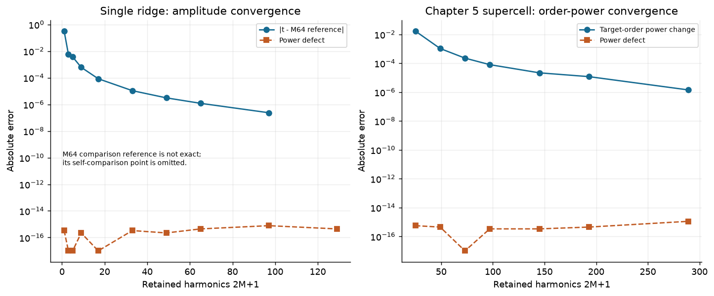
۵. تصمیم بازتولیدپذیر را حفظ کنید
سلول زیر آزمایش لایهٔ شما را جدا از ممیزی ثابت منتشرشده ذخیره میکند. شبکهٔ درشت مردود، شبکهٔ پذیرفتهشده، رواداری و کنترلهای مستقل دامنه و استخراج را گزارش کنید. برای پیکربندی فیزیکی جدید، موفقیت اعتبارسنج مرجع ثابت آزمایش تغییریافته را تأیید نمیکند. مدل همچنان جذب، نقشداربودن برداری، اثر دهانهٔ محدود و عدم قطعیت دادهٔ ماده را حذف میکند.
تمرین تکمیلی: زمان اجرا و جاذب FDTD را مستقل ریزسازی کنید؛ تیغهٔ فصل ۳ را در مدل FEM همگرا بازسازی کنید؛ اختلاف مدل تقریب ورقهٔ نازک را فقط با صفحههای فاز یکسان بسنجید. اینها طرح تمریناند و شبیهسازی انجامشده نیستند. منابع روش علمی و منشأ در data/chapter-06/README.md و فصل ثبت شدهاند.
experiment = {'parameters': asdict(SLAB), 'mesh':mesh, 'padding':padding,
              'criteria':{'complex_t':AMPLITUDE_TARGET,'phase_deg':PHASE_TARGET_DEG,'phase_amplitude_floor':PHASE_AMPLITUDE_FLOOR},
              'source_sha256':hashlib.sha256((ROOT/'simulations/numerical_methods.py').read_bytes()).hexdigest(),
              'scope':'1D lossless equal-exterior FDFD slab; RCWA figures use separate fixed datasets'}
destination = ROOT/'data/chapter-06/notebook-experiment.json'
destination.parent.mkdir(parents=True,exist_ok=True)
destination.write_text(json.dumps(experiment,indent=2,allow_nan=False)+'\n',encoding='utf-8')
print('Saved', destination.relative_to(ROOT))
Saved data\chapter-06\notebook-experiment.json