آیا شبکهٔ عصبی این جانشین را بهتر میکند؟
دفترچهٔ مقایسهٔ فصل ۱۰. ابتدا کرنل، سپس مقایسهٔ بازیابی، درونیابی خطی، KRR و MLP کوچک. فصل، آزمایشگاه و راهنما را بخوانید.
داده ورقهٔ تحلیلی مصنوعی است، نه حلگر تمامموج یا ساختار ساختهشده. دامنه و فرکانس بیبُعدند. پس از نصب requirements-labs.txt، دفترچه مستقل، بدون دادهٔ خارجی، GPU و شبکه اجرا میشود.
۱. پیش از برازش، آزمایش را اعلام کنید
۸۰ طرح، ۱۰۱ فرکانس، بذر ۲۴ و تقسیم طرح کامل ۴۰/۲۰/۲۰ آغازین.
انتخاب KRR از ۱۲ و MLP از ۶ نامزد با RMSE مختلط اعتبارسنجی؛ بودجه متفاوت است و معیار هزینهٔ برابر نیست.
انتخاب عصبی فقط با بذر ۲۴؛ سپس معماری و منظمسازی ثابت و تکرار ۴۲ و ۷۳. هر سه را گزارش و با آزمون بذر انتخاب نکنید.
مقیاس ورودی فقط با ۴۰ طرح آموزش. هدف ۱۰۱ حقیقی سپس ۱۰۱ موهومی؛ چون یک دامنهٔ محدود یکساناند، مقیاس نسبی جدا لازم نیست.
آموزش پس از انتخاب ثابت بماند؛ هیچ مدل با هدف اعتبارسنجی یا آزمون دوباره برازش نمیشود.
آزمون پس از تثبیت همهٔ مدلها آشکار شود. تقسیم تصادفی عمدتاً درونیابی خانوادهٔ یکبعدی است؛ تشخیص پوشش، حالت مرزی را نشان میدهد.
هر جانشین پیوسته ۹۰۱ مختصات یکسان و بازیابی یکی از ۴۰ طرح واقعی آموزش را میبیند. MLP بذر ۲۴، مستقل از رتبهٔ آزمون، در مقایسهٔ وارون استفاده شود.
MLP دارای tanh، خروجی خطی، L2 و L-BFGS است؛ اعتبارسنجی داخلی و توقف زودهنگام ندارد. هشدار و تعداد تکرار گزارش میشوند؛ API را ببینید.
این مقایسهٔ تدریسِ بازتولیدپذیر روی دادهٔ مصنوعی عمومی است، نه آزمون کور خصوصی. کد آزمون را از برازش و انتخاب جدا نگه میدارد. اگر پس از خواندن نتیجهٔ عمومی پروتکل را عوض کنید، برای ادعای تازه آزمایش کنارگذاشتهٔ تازه بسازید.
import sys
import warnings
import time
import numpy as np
import matplotlib
import matplotlib.pyplot as plt
import sklearn
import scipy
from sklearn.neural_network import MLPRegressor
from sklearn.preprocessing import StandardScaler
from sklearn.exceptions import ConvergenceWarning
from threadpoolctl import threadpool_limits
from IPython.display import display, HTML
from html import escape

SPLIT_SEED = 24
MLP_SEEDS = (24, 42, 73)
MLP_NAME = f"MLP (seed {MLP_SEEDS[0]})"
G_MIN, G_MAX, N_DESIGNS = 0.05, 0.95, 80
N_TRAIN, N_VALID = 40, 20
OMEGA_MIN, OMEGA_MAX, N_OMEGA = 0.8, 1.2, 101
OMEGA0_OFFSET, OMEGA0_SLOPE = 0.9, 0.2
GAMMA_OFFSET, GAMMA_SLOPE = 0.025, 0.02
LENGTH_SCALES = (0.03, 0.06, 0.12, 0.24)
KRR_ALPHAS = (1e-8, 1e-6, 1e-4)
MLP_LAYERS = ((16,), (32,), (32, 32))
MLP_ALPHAS = (1e-4, 1e-2)
MLP_MAX_ITER, MLP_MAX_FUN, MLP_TOL = 2000, 60000, 1e-8
PHASE_AMPLITUDE_MIN = 0.1
G_TARGET, N_CANDIDATES = 0.623, 901

assert 1 < N_TRAIN and 0 < N_VALID and N_TRAIN + N_VALID < N_DESIGNS
assert G_MIN < G_MAX and G_MIN <= G_TARGET <= G_MAX
assert OMEGA_MIN < OMEGA_MAX and N_OMEGA > 2 and N_CANDIDATES > 2
assert 0 < PHASE_AMPLITUDE_MIN < 1
assert len(set(MLP_SEEDS)) >= 3
assert all(x > 0 for x in (*LENGTH_SCALES, *KRR_ALPHAS, *MLP_ALPHAS))
print(f"Python {sys.version.split()[0]}; NumPy {np.__version__}; Matplotlib {matplotlib.__version__}; scikit-learn {sklearn.__version__}; SciPy {scipy.__version__}")
print("Synthetic analytical evidence only. One BLAS thread during training for a modest CPU workload.")

def table(headers, rows):
    # HTML tables render in both Jupyter and the static book's output viewer.
    header = "".join(f'<th scope="col">{escape(str(value))}</th>' for value in headers)
    body = "".join("<tr>" + "".join(f"<td>{escape(str(value))}</td>" for value in row) + "</tr>" for row in rows)
    display(HTML('<div style="overflow-x:auto;max-width:100%"><table><thead><tr>' +
                 header + '</tr></thead><tbody>' + body + '</tbody></table></div>'))
Python 3.12.1; NumPy 2.4.6; Matplotlib 3.11.1; scikit-learn 1.9.1; SciPy 1.18.1
Synthetic analytical evidence only. One BLAS thread during training for a modest CPU workload.
۲. بازتولید مولد و تقسیم
با ، محیط برابر و درگاه توانی:
بقا، تشدید و کل دودرگاه را بررسی کنید. برای علاوه بر ، شرط غیرقطری برای یکانی بودن لازم است. این کنترل مولد است، نه قید خودکار رگرسیون.
def resonant_sheet(g, omega):
    g = np.atleast_1d(np.asarray(g, dtype=float))[:, None]
    omega = np.atleast_1d(np.asarray(omega, dtype=float))[None, :]
    gamma = GAMMA_OFFSET + GAMMA_SLOPE * g
    if np.any(gamma <= 0):
        raise ValueError("The linewidth must be positive")
    delta = omega - (OMEGA0_OFFSET + OMEGA0_SLOPE * g)
    r = -gamma / (gamma - 1j * delta)
    return r, 1 + r

omega = np.linspace(OMEGA_MIN, OMEGA_MAX, N_OMEGA)
g_all = np.linspace(G_MIN, G_MAX, N_DESIGNS)
r_all, t_all = resonant_sheet(g_all, omega)
balance = np.abs(r_all)**2 + np.abs(t_all)**2 - 1
cross = np.conj(r_all) * t_all + np.conj(t_all) * r_all
assert np.max(np.abs(balance)) < 1e-12 and np.max(np.abs(cross)) < 1e-12
g_check = (G_MIN + G_MAX) / 2
r0, t0 = resonant_sheet(g_check, OMEGA0_OFFSET + OMEGA0_SLOPE*g_check)
assert np.allclose(r0, -1) and np.allclose(t0, 0)

ids = np.random.default_rng(SPLIT_SEED).permutation(N_DESIGNS)
train_ids = np.sort(ids[:N_TRAIN])
valid_ids = np.sort(ids[N_TRAIN:N_TRAIN + N_VALID])
test_ids = np.sort(ids[N_TRAIN + N_VALID:])
assert len(set(train_ids) & set(valid_ids)) == 0
assert len(set(train_ids) & set(test_ids)) == 0
assert len(set(valid_ids) & set(test_ids)) == 0
assert set(np.r_[train_ids, valid_ids, test_ids]) == set(range(N_DESIGNS))
g_train, y_train = g_all[train_ids], t_all[train_ids]
g_valid, y_valid = g_all[valid_ids], t_all[valid_ids]

print(f"Maximum generator balance residual: {np.max(np.abs(balance)):.3e}")
print(f"Maximum off-diagonal unitarity residual: {np.max(np.abs(cross)):.3e}")
for name, selection in [("Train", train_ids), ("Validation", valid_ids), ("Test", test_ids)]:
    outside = np.sum((g_all[selection] < g_train.min()) | (g_all[selection] > g_train.max()))
    print(f"{name}: IDs={selection.tolist()}; outside training-coordinate range={outside}")
Maximum generator balance residual: 5.551e-16
Maximum off-diagonal unitarity residual: 3.628e-16
Train: IDs=[0, 6, 7, 8, 11, 17, 22, 23, 25, 29, 31, 32, 33, 35, 36, 37, 38, 41, 42, 45, 49, 52, 53, 54, 56, 57, 58, 59, 61, 62, 63, 65, 66, 67, 68, 73, 75, 76, 77, 78]; outside training-coordinate range=0
Validation: IDs=[1, 2, 4, 10, 13, 16, 20, 21, 30, 34, 40, 43, 44, 46, 48, 50, 51, 69, 74, 79]; outside training-coordinate range=1
Test: IDs=[3, 5, 9, 12, 14, 15, 18, 19, 24, 26, 27, 28, 39, 47, 55, 60, 64, 70, 71, 72]; outside training-coordinate range=0
۳. بازیابی، درونیابی و کرنل
بازیابی نزدیکترین مختصات آموزشی را میگیرد. خطی، پرسش را بین مختصات آموزش قرار و دامنهٔ مختلط را مخلوط میکند، نه فاز پیچیده را. بیرون دامنه به انتها محدود میشود؛ تعداد پوشش، محدودیت را نشان میدهد. ابرپارامتر برازششده ندارد.
KRR همان دستگاه مختلط آغازین را حل و همهٔ امتیازهای اعتبارسنجی را حفظ میکند. هیچ نتیجهٔ این سلول از هدف آزمون استفاده نمیکند.
def complex_rmse(prediction, reference):
    return float(np.sqrt(np.mean(np.abs(prediction-reference)**2)))

def nearest_predict(g):
    nearest = np.argmin(np.abs(np.atleast_1d(g)[:, None]-g_train[None, :]), axis=1)
    return y_train[nearest]

def linear_predict(g):
    g = np.clip(np.atleast_1d(g), g_train[0], g_train[-1])
    right = np.clip(np.searchsorted(g_train, g, side="right"), 1, len(g_train)-1)
    left = right - 1
    fraction = ((g-g_train[left])/(g_train[right]-g_train[left]))[:, None]
    return (1-fraction)*y_train[left] + fraction*y_train[right]

def kernel(a, b, length):
    return np.exp(-0.5*((np.atleast_1d(a)[:, None]-np.atleast_1d(b)[None, :])/length)**2)

krr_trials = []
with threadpool_limits(limits=1):
    for length in LENGTH_SCALES:
        for alpha in KRR_ALPHAS:
            weights = np.linalg.solve(kernel(g_train, g_train, length)+alpha*np.eye(N_TRAIN), y_train)
            score = complex_rmse(kernel(g_valid, g_train, length) @ weights, y_valid)
            krr_trials.append((score, length, alpha, weights))
krr_score, best_length, best_alpha, krr_weights = min(krr_trials, key=lambda row: row[0])

def krr_predict(g):
    return kernel(g, g_train, best_length) @ krr_weights

table(["KRR length", "KRR alpha", "Validation complex RMSE"],
      [(length, f"{alpha:g}", f"{score:.6g}") for score, length, alpha, _ in krr_trials])
print(f"Selected KRR: length={best_length}, alpha={best_alpha:g}; validation RMSE={krr_score:.6g}")
assert np.allclose(linear_predict(g_train), y_train)
Selected KRR: length=0.12, alpha=1e-08; validation RMSE=0.000643005
۴. آموزش جانشین عصبی
یک لایه: و . خروجی حقیقی، است.
میانگین مربع روی مختصات نصف میانگین خطای مختلط روی فرکانس است. عامل ثابت رتبهٔ بدون منظمسازی را حفظ میکند، اما تفسیر زیان و منظمسازی مهم است. همه با RMSE مختلط یکسان پس از بازسازی انتخاب میشوند.
مقیاس یک بار با آموزش برازش میشود. وزن پنهان متغیر و مختصات طراحی ورودی ثابت است. L-BFGS برای دادهٔ کوچک انتخاب شده؛ هشدار باقی میماند و اجرای محدودشده را همگرا ننامید.
def pack(y):
    return np.concatenate([y.real, y.imag], axis=1)

def unpack(y):
    return y[:, :N_OMEGA] + 1j*y[:, N_OMEGA:]

assert np.allclose(unpack(pack(y_train)), y_train)
scaler = StandardScaler().fit(g_train[:, None])
x_train = scaler.transform(g_train[:, None])
x_valid = scaler.transform(g_valid[:, None])
assert np.allclose(scaler.mean_, np.mean(g_train))

def fit_mlp(layers, alpha, seed):
    model = MLPRegressor(hidden_layer_sizes=layers, activation="tanh", solver="lbfgs",
                         alpha=alpha, random_state=seed, max_iter=MLP_MAX_ITER,
                         max_fun=MLP_MAX_FUN, tol=MLP_TOL, early_stopping=False)
    start = time.perf_counter()
    with warnings.catch_warnings(record=True) as caught, threadpool_limits(limits=1):
        warnings.simplefilter("always")
        model.fit(x_train, pack(y_train))
    messages = [f"{w.category.__name__}: {w.message}" for w in caught]
    return model, messages, time.perf_counter()-start

mlp_trials = []
for layers in MLP_LAYERS:
    for alpha in MLP_ALPHAS:
        model, messages, seconds = fit_mlp(layers, alpha, MLP_SEEDS[0])
        score = complex_rmse(unpack(model.predict(x_valid)), y_valid)
        mlp_trials.append(dict(layers=layers, alpha=alpha, score=score, model=model,
                               warnings=messages, seconds=seconds))
        for message in messages:
            print(f"layers={layers}, alpha={alpha}: {message}")
chosen = min(mlp_trials, key=lambda row: row["score"])
table(["Hidden layers", "L2 alpha", "Validation complex RMSE", "Iterations", "Warnings"],
      [(row["layers"], row["alpha"], f'{row["score"]:.6g}', row["model"].n_iter_, len(row["warnings"]))
       for row in mlp_trials])

# Architecture/alpha selection is now frozen. Repeat seeds without any new selection.
seed_models = {MLP_SEEDS[0]: chosen["model"]}
seed_warnings = {MLP_SEEDS[0]: chosen["warnings"]}
for seed in MLP_SEEDS[1:]:
    model, messages, _ = fit_mlp(chosen["layers"], chosen["alpha"], seed)
    seed_models[seed], seed_warnings[seed] = model, messages
    for message in messages:
        print(f"Repeat seed={seed}: {message}")

def mlp_predict(g, seed=MLP_SEEDS[0]):
    return unpack(seed_models[seed].predict(scaler.transform(np.atleast_1d(g)[:, None])))

n_parameters = sum(array.size for array in (*chosen["model"].coefs_, *chosen["model"].intercepts_))
print(f'Selected MLP: layers={chosen["layers"]}, alpha={chosen["alpha"]}; parameters={n_parameters}')
print(f'Primary seed {MLP_SEEDS[0]}; repeats {MLP_SEEDS[1:]}. Models frozen before test evaluation.')
print(f'Total MLP selection fits={len(mlp_trials)}, repeat fits={len(MLP_SEEDS)-1}.')
layers=(16,), alpha=0.01: ConvergenceWarning: lbfgs failed to converge after 35 iteration(s) (status=2):
ABNORMAL:

You might also want to scale the data as shown in:
    https://scikit-learn.org/stable/modules/preprocessing.html
layers=(32,), alpha=0.01: ConvergenceWarning: lbfgs failed to converge after 53 iteration(s) (status=2):
ABNORMAL:

You might also want to scale the data as shown in:
    https://scikit-learn.org/stable/modules/preprocessing.html
layers=(32, 32), alpha=0.01: ConvergenceWarning: lbfgs failed to converge after 79 iteration(s) (status=2):
ABNORMAL:

You might also want to scale the data as shown in:
    https://scikit-learn.org/stable/modules/preprocessing.html
Selected MLP: layers=(32,), alpha=0.0001; parameters=6730
Primary seed 24; repeats (42, 73). Models frozen before test evaluation.
Total MLP selection fits=6, repeat fits=2.
۵. آشکار کردن آزمون کنارگذاشته
انتخابها ثابتاند. RMSE مختلط، MAE توان عبور بهصورت کسر مطلق، MAE دامنه، بدترین خطای نقطهای و MAE فاز دایروی با هر دو دامنه بالای ۰٫۱ و سهم حذف را گزارش کنید. حذف فاز، خطای دامنه را توجیه نمیکند.
فقط برای این ورقه، را بسازید و را گزارش کنید. باقیماندهٔ کم لزوماً طیف درست نیست؛ بازیابی میتواند تشدید غلط و بقای کامل داشته باشد. مخلوط خطی مختلط نیز ممکن است بیاتلاف بودن طیفهای انتها را نقض کند.
def metrics(prediction, reference):
    assert prediction.shape == reference.shape and np.isfinite(prediction).all()
    valid_phase = (np.abs(prediction) > PHASE_AMPLITUDE_MIN) & (np.abs(reference) > PHASE_AMPLITUDE_MIN)
    circular_error = np.abs(np.angle(prediction*np.conj(reference)))
    return dict(rmse=complex_rmse(prediction, reference),
                power_mae=float(np.mean(np.abs(np.abs(prediction)**2-np.abs(reference)**2))),
                amplitude_mae=float(np.mean(np.abs(np.abs(prediction)-np.abs(reference)))),
                max_complex_error=float(np.max(np.abs(prediction-reference))),
                phase_mae_deg=float(np.rad2deg(np.mean(circular_error[valid_phase]))) if valid_phase.any() else np.nan,
                excluded_pct=float(100*(1-valid_phase.mean())),
                balance_max=float(np.max(np.abs(np.abs(prediction-1)**2+np.abs(prediction)**2-1))))

predictors = {"Nearest": nearest_predict, "Linear": linear_predict, "KRR": krr_predict, MLP_NAME: mlp_predict}
g_test, y_test = g_all[test_ids], t_all[test_ids]
test_predictions = {name: predict(g_test) for name, predict in predictors.items()}
test_metrics = {name: metrics(pred, y_test) for name, pred in test_predictions.items()}
table(["Method", "Complex RMSE", "Power MAE", "Amplitude MAE", "Worst complex error"],
      [(name, *[f'{m[key]:.6g}' for key in ("rmse", "power_mae", "amplitude_mae", "max_complex_error")])
       for name, m in test_metrics.items()])
table(["Method", "Phase MAE (degrees)", "Phase excluded (%)", "Max balance residual"],
      [(name, f'{m["phase_mae_deg"]:.5g}', f'{m["excluded_pct"]:.4g}', f'{m["balance_max"]:.6g}')
       for name, m in test_metrics.items()])

seed_metrics = {seed: metrics(mlp_predict(g_test, seed), y_test) for seed in MLP_SEEDS}
table(["MLP seed", "Test complex RMSE", "Iterations", "Warnings"],
      [(seed, f'{seed_metrics[seed]["rmse"]:.6g}', seed_models[seed].n_iter_, len(seed_warnings[seed])) for seed in MLP_SEEDS])
seed_rmse = np.array([seed_metrics[seed]["rmse"] for seed in MLP_SEEDS])
print(f"MLP test RMSE across initializations: mean={seed_rmse.mean():.6g}; sample standard deviation={seed_rmse.std(ddof=1):.6g}")
print("Three initializations describe training variability on ONE fixed dataset split, not a confidence interval or split-generalization study.")
MLP test RMSE across initializations: mean=0.0231928; sample standard deviation=0.00732324
Three initializations describe training variability on ONE fixed dataset split, not a confidence interval or split-generalization study.
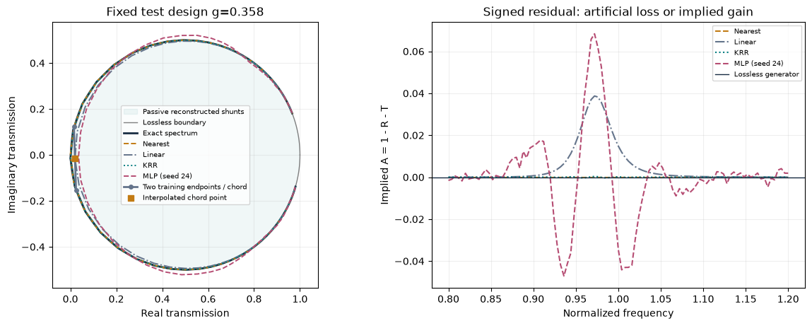
مکان هندسی عبور مختلط را بررسی کنید
فقط برای این ورقهٔ الکتریکی متقارن با دو محیط هوای یکسان، بازتاب را از عبور پیشبینیشده منهای یک بازسازی میکنیم. پاسخ بیاتلاف روی دایرهای با شعاع یکدوم و مرکز یکدوم در صفحهٔ عبور مختلط قرار دارد. داخل قرص، مدل بازسازیشده غیرفعال و دارای جذب مثبت است؛ بیرون آن مدل به بهره نیاز دارد.
درونیابی خطی مختلط پاسخهای دقیق آموزشی را با پارهخط وصل میکند. پارهخط در قرص غیرفعال میماند، ولی معمولاً دایرهٔ بیاتلاف را ترک میکند و اتلاف مصنوعی نسبت به مولد میافزاید. در مقابل، بازیابی نزدیکترین همسایه روی دایره میماند، حتی وقتی تشدید اشتباه را برمیگرداند. دقت پاسخ عددی و سازگاری فیزیکی به دو پرسش متفاوت پاسخ میدهند.
نمودار از شناسهٔ میانی آزمونِ مرتبشده و پیشبینیهای ثابت موجود استفاده میکند؛ انتخاب نمونه مستقل از خطاهای مدل است. باقیماندهٔ علامتدار، کنترل خروجی مدل بازسازیشده است و جذب اندازهگیریشدهٔ ماده نیست. جدول همهٔ هندسههای آزمون را نیز بررسی میکند. تصویر کردن پیشبینی روی دایره، دقت طیفی، علیت پهنباند یا تحققپذیری فیزیکی را اثبات نمیکند؛ آزمون قرص فقط به همین مدل و پایه محدود است.
# Reuse frozen predictions: no new fitting, model selection, or test-based tuning.
constraint_example = len(test_ids)//2
constraint_g = float(g_test[constraint_example])
constraint_colors = {'Nearest': '#c27b14', 'Linear': '#64748b', 'KRR': '#007d80', MLP_NAME: '#b64d73'}
constraint_styles = {'Nearest': '--', 'Linear': '-.', 'KRR': ':', MLP_NAME: '--'}
circle_angle = np.linspace(0., 2*np.pi, 401)
circle = .5+.5*np.exp(1j*circle_angle)
fig, axes = plt.subplots(1, 2, figsize=(11.5, 4.5), constrained_layout=True)
axes[0].fill(circle.real, circle.imag, color='#007d80', alpha=.06, label='Passive reconstructed shunts')
axes[0].plot(circle.real, circle.imag, color='.5', lw=1, label='Lossless boundary')
axes[0].plot(y_test[constraint_example].real, y_test[constraint_example].imag, color='#182c42', lw=2, label='Exact spectrum')
passivity_diagnostics = {}
for name, prediction in test_predictions.items():
    implied_absorption = 1-np.abs(prediction-1)**2-np.abs(prediction)**2
    circle_expression = .5-2*np.abs(prediction-.5)**2
    assert np.allclose(implied_absorption, circle_expression, rtol=1e-12, atol=1e-12)
    example_t = prediction[constraint_example]
    axes[0].plot(example_t.real, example_t.imag, constraint_styles[name], color=constraint_colors[name], lw=1.4, label=name)
    axes[1].plot(omega, implied_absorption[constraint_example], constraint_styles[name], color=constraint_colors[name], label=name)
    passivity_diagnostics[name] = dict(min_implied_absorption=float(implied_absorption.min()),
        max_implied_absorption=float(implied_absorption.max()),
        fraction_outside_passive_disk=float(np.mean(implied_absorption < -1e-9)))

# One interpolation chord at the frequency nearest this fixed design's resonance.
right = int(np.clip(np.searchsorted(g_train, constraint_g, side='right'), 1, len(g_train)-1))
left = right-1
chord_frequency = int(np.argmin(np.abs(omega-(OMEGA0_OFFSET+OMEGA0_SLOPE*constraint_g))))
chord = y_train[[left, right], chord_frequency]
axes[0].plot(chord.real, chord.imag, 'o-', color='#64748b', lw=2, ms=4, label='Two training endpoints / chord')
axes[0].scatter(test_predictions['Linear'][constraint_example, chord_frequency].real,
                test_predictions['Linear'][constraint_example, chord_frequency].imag,
                color='#c27b14', marker='s', s=34, zorder=5, label='Interpolated chord point')
axes[0].set(xlabel='Real transmission', ylabel='Imaginary transmission', aspect='equal',
            xlim=(-.08, 1.08), ylim=(-.58, .58), title=f'Fixed test design g={constraint_g:.3f}')
axes[1].axhline(0., color='#182c42', lw=1, label='Lossless generator')
axes[1].set(xlabel='Normalized frequency', ylabel='Implied A = 1 - R - T',
            title='Signed residual: artificial loss or implied gain')
for ax in axes:
    ax.grid(alpha=.2)
    ax.legend(fontsize=7, loc='best')
plt.show()
table(['Method', 'Minimum implied A', 'Maximum implied A', 'Outside passive disk (%)'],
      [(name, f'{v["min_implied_absorption"]:.6g}', f'{v["max_implied_absorption"]:.6g}',
        f'{100*v["fraction_outside_passive_disk"]:.4g}') for name, v in passivity_diagnostics.items()])
print('Signed diagnostics use every held-out design; the plot uses the predeclared middle sorted test ID.')
print('Positive implied A is artificial loss relative to this lossless generator; negative implied A indicates gain in the reconstructed shunt model.')
Signed diagnostics use every held-out design; the plot uses the predeclared middle sorted test ID.
Positive implied A is artificial loss relative to this lossless generator; negative implied A indicates gain in the reconstructed shunt model.
۶. خطا کجا رخ میدهد؟
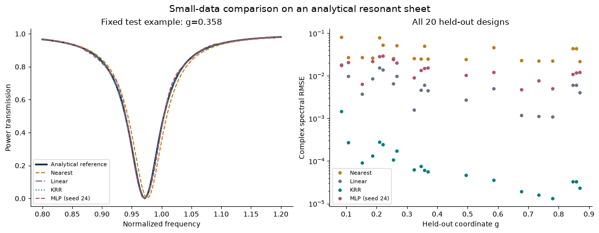
هندسهٔ نمونه با موقعیت در شناسههای مرتب آزمون از پیش ثابت است، نه با برندهٔ بعدی. نمودار پراکندگی همهٔ هندسهها را نشان میدهد. محور عمودی لگاریتمی است؛ عدد و منحنی را هر دو مقایسه کنید.
plt.rcParams.update({"font.size": 10, "axes.spines.top": False, "axes.spines.right": False})
colors = {"Nearest": "#c27b14", "Linear": "#64748b", "KRR": "#007d80", MLP_NAME: "#b64d73"}
styles = {"Nearest": "--", "Linear": "-.", "KRR": ":", MLP_NAME: "--"}
fig, axes = plt.subplots(1, 2, figsize=(12, 4.6), constrained_layout=True)
example = len(test_ids)//2
axes[0].plot(omega, np.abs(y_test[example])**2, color="#182c42", lw=2.5, label="Analytical reference")
for name, pred in test_predictions.items():
    axes[0].plot(omega, np.abs(pred[example])**2, styles[name], color=colors[name], label=name)
    error = np.sqrt(np.mean(np.abs(pred-y_test)**2, axis=1))
    axes[1].semilogy(g_test, np.maximum(error, 1e-16), "o", ms=4, color=colors[name], label=name)
axes[0].set(xlabel="Normalized frequency", ylabel="Power transmission", title=f"Fixed test example: g={g_test[example]:.3f}")
axes[1].set(xlabel="Held-out coordinate g", ylabel="Complex spectral RMSE", title=f"All {len(test_ids)} held-out designs")
axes[0].legend(fontsize=8)
axes[1].legend(fontsize=8)
fig.suptitle("Small-data comparison on an analytical resonant sheet", fontsize=14)
plt.show()
۷. پیشنهاد وارون در برابر مولد دقیق
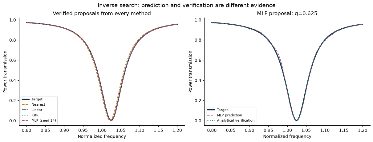
هدف قابلتحقق بسازید. هر روش طیف مختلط و شبکهٔ کراندار یکسان را میبیند؛ مختصات هدف به جستوجو داده نمیشود. در مختصات انتخابی، مولد تحلیلی و RMSE هدف پیشبینی و بررسی را حساب کنید.
بازیابی ناحیهٔ هدف تخت دارد، چون یک طیف آموزشی را برای بازهٔ پرسش برمیگرداند. برای پرهیز از هندسهٔ خیالی، نامزد آن مختصات واقعی آموزشی با کمترین اختلاف هدف است. ۴۰ نامزد کتابخانه زیرمجموعهٔ اطلاعات جستوجوی ۹۰۱ شبکهای جانشین پیوستهاند؛ شمار و تفکیک صریح چاپ میشوند.
هدف اتفاقاً روی شبکه است و خطای بررسی صفر ممکن است؛ بهینهٔ جهانی پیوسته یا عملکرد خانوادهٔ نامعلوم را ثابت نمیکند.
_, target = resonant_sheet(G_TARGET, omega)
g_candidates = np.linspace(G_MIN, G_MAX, N_CANDIDATES)
inverse_results = {}
for name, predict in predictors.items():
    candidates = g_train if name == "Nearest" else g_candidates
    spectra = predict(candidates)
    objectives = np.mean(np.abs(spectra-target)**2, axis=1)
    selected = int(np.argmin(objectives))
    g_selected = float(candidates[selected])
    predicted = spectra[selected:selected+1]
    r_verified, verified = resonant_sheet(g_selected, omega)
    assert G_MIN <= g_selected <= G_MAX and np.isfinite(objectives).all()
    assert np.max(np.abs(np.abs(r_verified)**2+np.abs(verified)**2-1)) < 1e-12
    inverse_results[name] = dict(g=g_selected, predicted=predicted, verified=verified,
                                 predicted_rmse=complex_rmse(predicted, target),
                                 verified_rmse=complex_rmse(verified, target))
table(["Method", "Selected g", "Predicted target RMSE", "Verified target RMSE"],
      [(name, f'{r["g"]:.6f}', f'{r["predicted_rmse"]:.6g}', f'{r["verified_rmse"]:.6g}')
       for name, r in inverse_results.items()])
print(f"Target g={G_TARGET}; continuous-surrogate grid={N_CANDIDATES}; spacing={g_candidates[1]-g_candidates[0]:.6g}; retrieval candidates={len(g_train)}")

fig, axes = plt.subplots(1, 2, figsize=(12, 4.5), constrained_layout=True)
axes[0].plot(omega, np.abs(target[0])**2, color="#182c42", lw=2.5, label="Target")
for name, result in inverse_results.items():
    axes[0].plot(omega, np.abs(result["verified"][0])**2, styles[name], color=colors[name], label=name)
mlp_result = inverse_results[MLP_NAME]
axes[1].plot(omega, np.abs(target[0])**2, color="#182c42", lw=2.5, label="Target")
axes[1].plot(omega, np.abs(mlp_result["predicted"][0])**2, "--", color="#b64d73", label="MLP prediction")
axes[1].plot(omega, np.abs(mlp_result["verified"][0])**2, ":", color="#007d80", lw=2, label="Analytical verification")
axes[0].set(title="Verified proposals from every method", xlabel="Normalized frequency", ylabel="Power transmission")
axes[1].set(title=f'MLP proposal: g={mlp_result["g"]:.3f}', xlabel="Normalized frequency", ylabel="Power transmission")
for ax in axes:
    ax.legend(fontsize=8)
fig.suptitle("Inverse search: prediction and verification are different evidence", fontsize=13)
plt.show()
Target g=0.623; continuous-surrogate grid=901; spacing=0.001; retrieval candidates=40
۸. تفسیر، بازتولید و گسترش
پیش از تغییر از جدولها پاسخ دهید: کدام RMSE کمترین است و آیا با بدترین خطا یا بقا رتبه عوض میشود؟ آیا MLP از بازیابی، خطی و KRR بهتر است؟ پاسخ منفی علمی معتبر است. تغییر مقداردهی در برابر فاصلهٔ روشها چقدر و آیا سه بذر رتبهٔ عمومی دادههای دیگر را توجیه میکند؟ کدام وارون کمترین خطای بررسیشده و چرا متفاوت با پیشبینی است؟ چرا بازیابی میتواند با بقای عالی هدف را بد تطبیق دهد؟
شناسه، همهٔ نامزدها، انتخاب، وضعیت بهینهساز، سه اجرای عصبی، دو جدول آزمون و وارون پیشبینی و بررسی را نگه دارید؛ هشدار را با شل کردن بیخبر معیار حذف نکنید.
توسعه، آزمایش تازه است. پیش از مشاهدهٔ آزمون، پروتکل آموزش کمتر، بازهٔ کامل کنارگذاشته، پهنا یا نویز مختلط مستند را اعلام و از مرجع جدا کنید. پس از تنظیم روی آزمون منتشرشده، آن را دستنخورده ننامید.
گام قطعه، مرحلهٔ ب با کتابخانهٔ تمامموج همگرا، مخرج و تقسیم هندسهای است. این نتایج تحلیلی، ساخت، دقت تمامموج، افزایش سرعت محاسباتی یا برتری جهانی هیچ مدل را نشان نمیدهند.